Adaptively Refined Large-Eddy Simulations of Galaxy Clusters 8 Cluster physics 10 Summary and Conclusions

Chapter 9 Simulations of galaxy clusters

9.1 Details of the simulations

We performed two simulations of cluster formation with Enzo following Iapichino and Niemeyer (2008). One simulation was done with the Schmidt SGS model including the Sarkar corrections and some additional modifications described below. For comparsion we conducted a second simulation without SGS model. In the following section we describe the common features of these two simulations, in section 9.1.2 we describe some additional numerical issues, which had to be taken into account when doing a cluster simulation with SGS model in comoving coordinates.

9.1.1 Common features

The simulations were done using a flat (critical density $\Omega=1$ ) cold dark matter (CDM) background cosmology with a dark energy density $\Omega_{\Lambda}=0.7$ , a total (including baryonic and dark matter) matter density $\Omega_{m}=0.3$ , a baryonic matter density $\Omega_{b}=0.04$ , the Hubble parameter set to $h=0.7$ , a galaxy fluctuation amplitude $\sigma_{8}=0.9$ , and a scalar spectral index $n=1$ . Both simulations were started with the same initial conditions at redshift $z_{ini}=60$ , using the Eisenstein and Hu (1999) transfer function, and evolved to $z=0$ . The simulations were adiabatic with a heat capacity ratio $\gamma=5/3$ assuming a fully ionized gas with a mean molecular weight $m_{\mu}=0.6\,\mathrm{u}$ . Cooling physics, magnetic fields, feedback, and transport processes are neglected.

The simulation box had a comoving size of $128\,\mathrm{Mpc\ h^{-1}}$ . It was resolved with a root grid (level $l=0$ ) of $128^{3}$ cells and $128^{3}$ N-body particles. A static child grid ( $l=1$ ) was nested inside the root grid with a size of 64 Mpc/h, $128^{3}$ cells and $128^{3}$ N-body particles. The mass of each particle in this grid was $9\times 10^{9}\,\mathrm{M_{\odot}\ h^{-1}}$ . Inside this grid, in a volume of $38.4\,\mathrm{Mpc\ h^{-1}}$ , adaptive grid refinement from level $l=2$ to $l=6$ was enabled using a overdensity refinement criteria as described in Iapichino and Niemeyer (2008) with an overdensity factor $f=4.0$ . The refinement factor between two levels was set to $r=2$ , allowing for a effective resolution of $8196^{3}$ cells or $15.6\,\mathrm{kpc\ h^{-1}}$ .

The static and dynamically refined grids were nested around the place of formation of a galaxy cluster, identified by Iapichino and Niemeyer (2008) using the HOP algorithm (Eisenstein and Hut, 1998). The cluster had a virial mass of $M_{vir}=5.49\times 10^{14}\,\mathrm{M_{\odot}\ h^{-1}}$ and a virial radius of $R_{vir}=1.33\,\mathrm{Mpc\ h^{-1}}$ for both simulations.

9.1.2 Numerical issues

Running robust simulations including a SGS model like the Schmidt or Sarkar model in a comoving cosmological background requires some additional techniques not yet discussed. Apart from the additional terms due to comoving coordinates in the filtered equations, these techniques help to handle the extreme high turbulent Mach numbers, which appear on the coarsest grids in these simulations and are briefly described in the following sections.

Filtered equations of fluid dynamics in comoving coordinates

Filtering the equations of fluid dynamics in comoving coordinates (H.25)-(H.27) can be done in the same way as filtering the equations in cartesian coordinates as shown in chapter 4. As a result we get

$\displaystyle\frac{\partial}{\partial t}\langle\tilde{\rho}\rangle+\frac{1}{a}% \frac{\partial}{\partial x_{j}}\hat{u}_{j}\langle\tilde{\rho}\rangle=$	$\displaystyle 0,$		(9.1)
$\displaystyle\begin{split}\displaystyle\frac{\partial}{\partial t}\langle% \tilde{\rho}\rangle\hat{u}_{i}+\frac{1}{a}\frac{\partial}{\partial x_{j}}\hat{% u}_{j}\langle\tilde{\rho}\rangle\hat{u}_{i}=&\displaystyle-\frac{1}{a}\frac{% \partial}{\partial x_{i}}\langle\tilde{p}\rangle+\frac{1}{a}\frac{\partial}{% \partial x_{j}}\langle\sigma^{\prime}_{ij}\rangle+\langle\tilde{\rho}\rangle% \hat{g}^{*}_{i}-\frac{1}{a}\frac{\partial}{\partial x_{j}}\hat{\tau}(u_{i},u_{% j})\\ &\displaystyle-\frac{\dot{a}}{a}\langle\tilde{\rho}\rangle\hat{u}_{i},\end{split}$		(9.2)
$\displaystyle\begin{split}\displaystyle\frac{\partial}{\partial t}\langle% \tilde{\rho}\rangle e_{res}+\frac{1}{a}\frac{\partial}{\partial x_{j}}\hat{u}_% {j}\langle\tilde{\rho}\rangle e_{res}=&\displaystyle-\frac{1}{a}\frac{\partial% }{\partial x_{i}}\hat{u}_{i}\langle\tilde{p}\rangle+\frac{1}{a}\frac{\partial}% {\partial x_{j}}\hat{u}_{i}\langle\sigma^{\prime}_{ij}\rangle+\frac{1}{a}% \langle\tilde{\rho}\rangle\hat{u}_{i}\hat{g}^{*}_{i}\\ &\displaystyle-\frac{\dot{a}}{a}(\langle\tilde{\rho}\rangle e_{res}+\frac{1}{3% }\langle\tilde{\rho}\rangle\hat{u}_{i}\hat{u}_{i}+\langle\tilde{p}\rangle)\\ &\displaystyle+\langle\tilde{\rho}\rangle(\lambda+\epsilon)-\frac{1}{a}\hat{u}% _{i}\frac{\partial}{\partial x_{j}}\hat{\tau}(u_{i},u_{j})-\frac{1}{a}\frac{% \partial}{\partial x_{j}}\hat{\tau}(u_{j},e_{int}),\end{split}$		(9.3)
$\displaystyle\frac{\partial}{\partial t}\langle\tilde{\rho}\rangle e_{t}+\frac% {1}{a}\frac{\partial}{\partial x_{j}}\hat{u}_{j}\langle\tilde{\rho}\rangle e_{% t}=$	$\displaystyle\mathbb{D}+\Gamma-\langle\tilde{\rho}\rangle(\lambda+\epsilon)-% \frac{1}{a}\hat{\tau}(u_{j},u_{i})\frac{\partial}{\partial x_{j}}\hat{u_{i}}-2% \frac{\dot{a}}{a}\langle\tilde{\rho}\rangle e_{t}.$		(9.4)

In the source code of Enzo the derivatives are always taken with respect to $r_{i}=ax_{i}$ and the additional terms due to comoving coordinates in momentum and resolved energy equation are already implemented. So the only term we had to implement additionally compared to the non-comoving case was the term $2\frac{\dot{a}}{a}\langle\tilde{\rho}\rangle e_{t}$ in the equation of turbulent energy. Furthermore for the subgrid model terms it is necessary to take into account that the Jacobian of the velocity in comoving coordinates is⁴³⁴³See equation (H.7) in the Appendix.

\displaystyle J_{ij}=\frac{\partial}{\partial r_{i}}v_{j}

\displaystyle=\frac{1}{a}\frac{\partial}{\partial x_{i}}u_{j}+\frac{\dot{a}}{a% }\delta_{ij}.

(9.5)

The tracefree rate of strain tensor in comoving coordinates for example can then be easily expressed in terms of the Jacobian of the velocity field

\displaystyle S^{*}_{ij}=\frac{1}{2}{\left(J_{ij}+J_{ji}\right)}-\frac{1}{3}% \delta_{ij}J_{kk}.

(9.6)

Basically all terms in the subgrid model using derivatives of the resolved velocity are therefore written in terms of the Jacobian of the velocity.

Turbulent energy cutoff and lower limit for temperature

High turbulent Mach numbers occur in cosmological simulations especially in the very cold, low-density voids of the computational domain. To make sure that in our adiabatic simulation the temperature and therefore the sound speed doesn’t drop to unphysical low values we introduced a lower limit of the temperature $T_{min}=10\,\mathrm{K}$ . This value is reasonable, since no gas in the universe can have a temperature lower than the cosmic microwave background temperature of 2.7 K for a longer time. Since there are presumably more heating mechanisms like UV-heating, choosing 10 K as a lower limit seems to be a rational choice.

On the other side, low density gas can be accelerated very quickly in a gravitating field, leading to high velocity gradients, which lead to production of high amounts of turbulent energy according to the turbulent viscosity hypothesis. However the validity of the turbulent viscosity hypothesis has never been tested or verified in astrophysical flows. We are therefore free to assume that for flows with high velocity gradients, the production of turbulent energy is restricted and use as an upper limit of the turbulent Mach number $M_{t,max}=\sqrt{2}$ . The exact value of this limit is based on the idea that in an isothermal gas (speed of sound $c_{\text{s,iso}}=\frac{p_{th}}{\rho}$ ), the total pressure can be expressed as

\displaystyle p_{tot}=\rho c_{\text{s,iso}}^{2}+\frac{1}{3}\rho q^{2}=\gamma_{% \text{eff}}\rho c_{\text{s,iso}}^{2}.

(9.7)

If we assume that $\gamma_{\text{eff}}$ is not allowed to be higher than the adiabatic value $\gamma=5/3$ , we have to limit the isothermal turbulent Mach number to $\frac{q}{c_{\text{s,iso}}}\leq\sqrt{2}$ .

Treatment of shocks

Shocks form unavoidably during cosmological structure formation due to infalling plasma which accretes onto filaments, sheets, and halos, as well as due to supersonic flows associated with merging substructures (Pfrommer et al., 2006). But shocks are the most localized and anisotropic features of a flow and therefore cannot be treated by an SGS model, which is based on the assumption of isotropy of the flow on the subgrid scales.⁴⁴⁴⁴Also see chapter 6. So in principle, shocks should be treated by the mechanisms of AMR alone and the SGS model should not influence the shocks. That’s why we implemented a simple shock detector

\displaystyle-\frac{\partial v_{i}}{\partial r_{i}}l_{\Delta}>c_{s},

(9.8)

which marks all cells, where the velocity increments are greater than the speed of sound, as shocks. At these cells, we disable the SGS model, which means no production or dissipation of turbulence takes place. The turbulent energy is only advected in these cells.

9.2 Results

9.2.1 Energy conservation

Energy conservation is crucial for any adiabatic fluid dynamic simulation. However it is difficult to test for this directly in our setup, since we cannot extract easily the energy injected by gravity into the system. By plotting the time development of the mass weighted mean total energy in the system, which is for the simulation without SGS model the sum of mass weighted mean internal energy and mass weighted mean kinetic energy and for the simulation with Sarkar model the sum of mass weighted means of internal, kinetic and turbulent energy, we can still gain some insights into the differences between the two simulations.

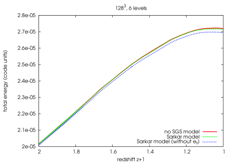
Figure 9.1: Time development of total energy in cluster simulation with and without SGS model.

This is what has been done in figure 9.1. From it we can see that the time development of the total energy is nearly identical, if we take the turbulent energy into account when computing the total energy of the simulation with Sarkar model. On the other side, the difference between the sum of kinetic and internal energy between the simulations seems to be again mostly accounted for by the turbulent energy, a result similar to what was already found in the simulations of driven turbulence.⁴⁵⁴⁵See section 7.3. We can also infer from figure 9.1, that the SGS model mainly changes the ratio of mean internal to mean kinetic energy and does not have much influence on the mean potential energy of the system. However, this is to be expected, since most of the gravitational potential is due to dark matter anyway, and we do not model the influence of gravity on subgrid scales and vice versa in our SGS model. This leads us to conclude that the general effects of our SGS model in a selfgravitating fluid are very similar to the effects found in the driven turbulence simulations without self gravity.

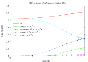
9.2.2 Mass fractions of different gas phases

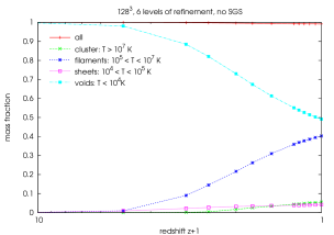
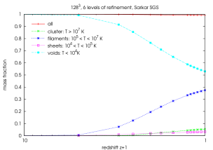
The IGM on large scales of the universe can be classified roughly into four phases according to gas temperature: the hot gas with $T>10^{7}\,\mathrm{K}$ inside and around clusters; the warm-hot intergalactic medium (WHIM) with $10^{5}\,\mathrm{K}<T<10^{7}\,\mathrm{K}$ found mostly in filaments; the low temperature WHIM with $10^{4}\,\mathrm{K}<T<10^{5}\,\mathrm{K}$ distributed mostly as sheetlike structures; and the diffuse cold gas with $T<10^{4}\,\mathrm{K}$ residing mostly in voids (Cen and Ostriker, 1999; Kang et al., 2005). To investigate the influence of the SGS model on these different gas phases, we plotted the time development of the mass fractions according to each of the phase for the simulation with and without SGS model (figure a and b).

We also show the mass fractions of each gas phase at redshift $z=0$ in table 9.1.

Run	$\frac{m_{\text{cluster}}}{m_{\text{all}}}\ [\%]$	$\frac{m_{\text{filaments}}}{m_{\text{all}}}\ [\%]$	$\frac{m_{\text{sheets}}}{m_{\text{all}}}\ [\%]$	$\frac{m_{\text{voids}}}{m_{all}}\ [\%]$
no SGS	5.50	40.3	4.22	49.1
SGS	5.47	37.5	3.28	53.0

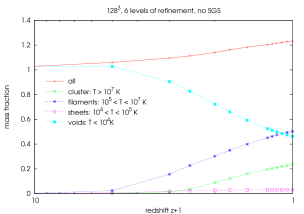
Table 9.1: Mass fractions of different gas phases at redshift

z=0

The results seem to indicate that the SGS model leads to higher mass fraction of the voids and a lower mass fraction of the filaments compared to the simulation without SGS model. However our simulation domain is not very well resolved outside the central region, since we do not allow for adaptive refinement there. If we restrict our analysis to the adaptively refined region in the box with a size of $38.4\,\mathrm{Mpc\ h^{-1}}$ , the differences between the simulation with SGS model and without SGS model vanish (figure a and b).

This can also be seen from the mass fractions at redshift $z=0$ normalized to the total mass in the central region in table 9.2.

Run	$\frac{m_{\text{cluster}}}{m_{\text{all}}}\ [\%]$	$\frac{m_{\text{filaments}}}{m_{\text{all}}}\ [\%]$	$\frac{m_{\text{sheets}}}{m_{\text{all}}}\ [\%]$	$\frac{m_{\text{voids}}}{m_{all}}\ [\%]$
no SGS	19.2	40.8	2.61	37.5
SGS	19.0	40.1	2.64	38.2

Table 9.2: Mass fractions of different gas phases at redshift

z=0

for the adaptively refined region with a size of

38.4\,\mathrm{Mpc\ h^{-1}}

From these results we conclude that the SGS model has no or only very little influence on the mass fractions of the different gas phases in the simulations. For the important mass fraction of the WHIM we get $\approx 38\%$ , which is higher than found by Davé et al. (2001, simulation B1) ( $\approx 32\%$ ) with a lower resolution AMR simulation, but lower than found by Gottlöber et al. (2006) ( $\approx 40\%$ ), who used smoothed particle hydrodynamic (SPH) with $2\times 1024^{3}$ particles to simulate a box of size $500\,\mathrm{Mpc\ h^{-1}}$ ; so we are also consistent with the literature in this respect.

9.2.3 Development of turbulence in different gas phases

The eddy turnover time $t_{l}$ associated with a scale $l$

\displaystyle t(l)=\frac{l}{q(l)}

(9.9)

is the typical time for a structure of size $\sim l$ to undergo a significant distortion due to turbulent motions characterized by the typical turbulent velocity $q(l)$ at that scale (Frisch, 1995). So if we divide the age of the universe $t(z)$ by the eddy turnover time, we get the number of eddy turnovers

\displaystyle n(l,z)=\frac{t(z)}{t(l)}

(9.10)

at a given redshift $z$ at a scale $l$ . If $n>1$ , there has been enough time for eddies of size $l$ to cascade down to smaller scales and we can call the fluid turbulent at scale $l$ .

In static grid simulations one often chooses to use the grid resolution $l_{\Delta}$ as characteristic length scale and to compute a characteristic velocity and eddy turnover time for this scale. However in an AMR code it is not trivial to compute the turbulent velocity $q_{l}$ associated with a characteristic length scale $l=l_{\Delta}$ , since $l_{\Delta}$ is varying in time and space. To circumvent this difficulty, we assume that below the grid resolution at a certain position turbulent velocity scales according to Kolmogorov

\displaystyle q(l)\sim l^{1/3}.

(9.11)

We thereby assume that locally, the cascade starts at a different length scale characterized by the different resolution of our grid at that position. We also assume that our refinement criterion tracks and finds the regions inside the fluid, which do not scale according to Kolmogorov, and refines them until a Kolmogorov scaling is reached. Of course one might doubt that our refinement criterion based on overdensity will accomplish that. But since in cosmological simulations gravity is basically the energy-injecting force in the fluid and gravity is strongest in regions of high density, one can argue that in regions of high density, the Kolmogorov cascade starts at smaller length scales and the energy injecting scales in these regions have to be refined with a finer grid. Of course a criterion solely based on density might be necessary, but is not at all sufficient to track regions of Non-Kolmogorov scaling. More research needs to be done in this direction, but it is outside of the scope of this work.

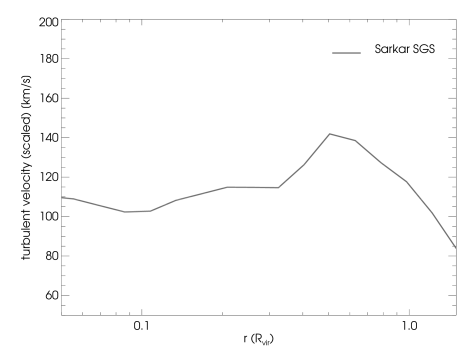
For the analysis in our work, we adopt the hypothesis of local Kolmogorov scaling below the grid resolution. As a characteristic scale of our analysis, we choose the length scale of our highest resolved regions, which is $l_{min}=15.6\,\mathrm{kpc\ h^{-1}}$ . The turbulent velocity in the highest resolved regions can be directly computed from the values of the turbulent energy $q(l)=\sqrt{2e_{t}}$ on the grid; the turbulent velocity in less refined regions is scaled down according to our local Kolmogorov hypothesis as

\displaystyle q(l_{min})=q(l_{\Delta}){\left(\frac{l_{min}}{l_{\Delta}}\right)% }^{1/3}.

(9.12)

Using this scaled turbulent velocity to compute the eddy turnover time, we plotted the mean mass weighted number of eddy turnovers at $l_{min}$ with respect to redshift (see figure 9.4).

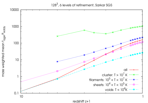
Figure 9.4: Mean number of eddy turnovers for gas phases of different temperature over time.

We can clearly see from this graph, that starting from a redshift $z=2$ all gas phases are turbulent at the scale $l_{min}=15.6\,\mathrm{kpc\ h^{-1}}$ . We also see that the amount of turbulence in terms of eddy turnover times is higher in regions of higher temperature and therefore highest in the cluster gas.

Another important measure for turbulence is the turbulent Mach number introduced in section 5.3.2. Like the eddy turnover time, the turbulent Mach number is scale dependent

\displaystyle M_{t}(l)=\frac{q(l)}{c_{s}}.

(9.13)

In figure 9.5 we plot the mean mass weighted turbulent Mach number characteristic for the scale of our analysis $l_{min}=15.6\,\mathrm{kpc\ h^{-1}}$ making again use of our local Kolmogorov hypothesis.

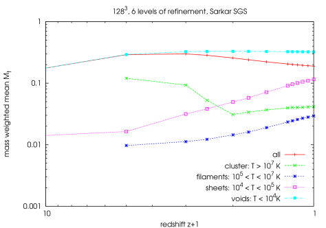
Figure 9.5: Mean turbulent Mach number at a scale $l_{min}=15.6\,\mathrm{kpc\ h^{-1}}$ for gas phases of different temperature over time.

It is evident that the turbulence at $l_{min}$ is subsonic in all gas phases during the whole time of the simulation. At redshift $z=0$ the average turbulent Mach number is $\approx 0.2$ . If the amount of turbulence would be equal in each gas phase one would expect the turbulent Mach number to scale $\sim 1/c_{s}\sim 1/\sqrt{T}$ . However this is not the case. The cluster gas is much more turbulent than estimated by this simple scaling relation; in fact there is more turbulent energy compared to internal energy in the hottest gas phase than in the WHIM, although there is a substantial drop of the turbulent Mach number between redshift $z=1-2$ . The drop in turbulent Mach number is presumably due to heating of the cluster gas during a phase of major mergers at that time. In the next section, we will present some further evidence for this interpretation.

9.2.4 Scaling of turbulent energy

In chapter 7 we studied the scaling of the turbulent energy with the resolution and were able to show that the scaling of turbulent energy in our simulations of driven turbulence actually follows the Kolmogorov scaling law. In this section we repeat this analysis for our cluster simulation. Figure 9.6 shows the time development of the mass weighted mean turbulent energy for every level of our AMR simulation.

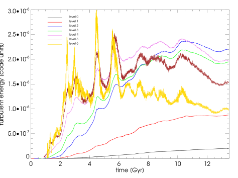
Figure 9.6: Time development of mean turbulent energy over time for each level of refinement.

We see from the plot, that the turbulent energy on the higher levels (meaning at smaller scales) is higher at times $t<6\,\mathrm{Gyr}$ . Later this picture changes, but not completely. For example the turbulent energy on level 4 stays above the turbulent energy of level 3 for the whole simulation time. Also striking are the high fluctuations in the time $2\,\mathrm{Gyr}<t<6\,\mathrm{Gyr}$ , which correspond to a redshift $z=3-1$ of the turbulent energy at the smaller scales. This is also the time when the turbulent Mach number inside the cluster drops significantly (see last section), so we can interpret these high fluctuations as further evidence for violent major mergers, that happen at that time, producing turbulent energy, which is then dissipated into internal energy heating up the cluster gas. However at the time $t>13\,\mathrm{Gyr}$ , the simulation seems to reach some kind of stable state, similar to what is found in driven turbulence simulations. We therefore can compute mean turbulent energies by averaging the turbulent energy from $t=13\,\mathrm{Gyr}$ to the end of the simulation and plot them against the grid length scale of the associated level. The result (in terms of the turbulent velocity) can be seen in figure 9.7.

Figure 9.7: Scaling of mean turbulent energy. The dotted line is a fit showing the scaling behavior of turbulent energy below $100\,\mathrm{kpc\ h^{-1}}$ , the dashed line is a fit showing the scaling behavior above $100\,\mathrm{kpc\ h^{-1}}$ .

It is obvious that this is no Kolmogorov scaling. However, we do not expect to see a Kolmogorov scaling again, since, as explained in the last section, we assume the resolved regions to be non-Kolmogorov anyway. Still the result is interesting, showing a peak in the turbulence around $100\,\mathrm{kpc\ h^{-1}}$ and a drop off towards higher and smaller scales. Also shown in the figure are power-law fits, which gave a scaling of $q\sim l^{-0.78}$ for scales bigger than $100\,\mathrm{kpc\ h^{-1}}$ and a scaling of $q\sim l^{0.24}\sim l^{1/4}$ for smaller scales. If one wants to interpret this result in terms of a turbulent cascade, one could say that up to a length scale of $100\,\mathrm{kpc\ h^{-1}}$ , energy is injected into the system, cascading down towards smaller scales with a scaling behavior $q\sim l^{1/4}$ flatter than expected for a Kolmogorov scaling with $q\sim l^{1/3}$ . But, assuming our local Kolmogorov hypothesis holds, it would follow, that below the grid resolution of $15.7\,\mathrm{kpc\ h^{-1}}$ the cascade should be Kolmogorov again. Of course a interpretation like this is highly speculative; much more data on turbulence in cluster simulations is necessary to show that the observed power-law scalings are real indeed.

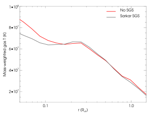
9.2.5 Radial profiles of the cluster

As mentioned in section 9.1.1, the simulation is centered around a galaxy cluster with a virial mass of $M_{vir}=5.49\times 10^{14}\,\mathrm{M_{\odot}\ h^{-1}}$ and a virial radius of $R_{vir}=1.33\,\mathrm{Mpc\ h^{-1}}$ for both simulations, which center is identified using the HOP algorithm. In the following we present plots of radial profiles of several quantities around the center of this cluster (figure a-c) obtained by using a modified version⁴⁶⁴⁶We modified enzo_anyl to allow plotting of SGS model quantities like the turbulent velocity. of the enzo_anyl tool, which is part of the public Enzo release.

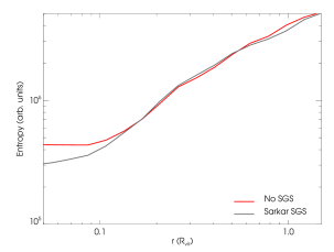
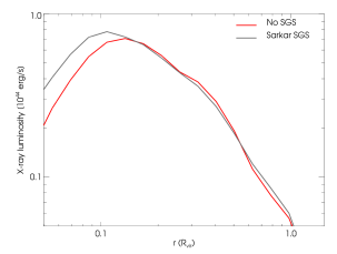
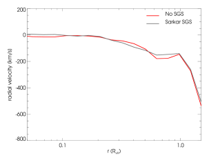
The plots show the mass weighted average values at radius $r$ of temperature $T(r)$ in Kelvin, the density⁴⁷⁴⁷The density is not mass weighted . $\rho(r)$ in $\mathrm{M_{\odot}/Mpc^{3}}$ , the scaled turbulent velocity according to equation (9.12) $v_{t}(r)$ in $\mathrm{km\ s^{-1}}$ , the radial component of the resolved velocity $v_{r}(r)$ in $\mathrm{km\ s^{-1}}$ , the entropy $K$ in code units, which is defined as⁴⁸⁴⁸This definition of entropy is often used in literature on galaxy clusters (Voit, 2005; Iapichino and Niemeyer, 2008).

\displaystyle K=\frac{T}{\rho^{\gamma-1}}

(9.14)

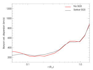
with $\gamma=5/3$ , the x-ray luminosity $L_{X}\sim\rho^{2}T^{1/2}$ and the radially averaged velocity dispersion, which is defined as the standard deviation of the velocity averaged over a spherical shell as

\displaystyle\sigma(r)=\frac{\sum_{i}m_{i}{\left(v_{i}-\langle v(r)\rangle% \right)}^{2}}{\sum_{i}m_{i}}

(9.15)

where $\langle v(r)\rangle=\frac{\sum_{i}m_{i}}{\sum_{i}m_{i}}$ is the mass weighted mean value of velocity in the spherical shell at radius $r\pm\delta r$ .

At first it is apparent from these plots that, except for the radial component of the resolved velocity, the run with SGS model only shows significant deviations from the run without SGS model in the cluster core at $r<0.1\ R_{vir}$ . However since enzo_anyl proved not to be robust for $r<0.07\ R_{vir}$ (Iapichino and Niemeyer, 2008), one cannot use the values obtained by these plots for a consistent analysis of the cluster core; this will be done in the next chapter using a different tool. Nevertheless the general trend from these plots is, that the SGS model lowers the entropy in the core, which leads to a higher density and a lower temperature in the center of the cluster. Since the X-ray luminosity is proportional to $\rho^{2}$ , it is higher in the cluster core of the simulation with SGS model. Looking more precisely at the radial profile of entropy (fig. c), one can also see that in the simulation without the SGS model, the entropy inside the core of the cluster $r>0.1\ R_{vir}$ is basically constant, which suggests that the gas is adiabatic there. With the SGS model this is not the case; the entropy is falling steadily towards the center of the core.

The last observation can be discussed more quantitatively in terms of polytropic processes. A polytropic process is defined as a process, where

\displaystyle\frac{T}{\rho^{n-1}}=const.,

(9.16)

where $n$ is called the polytropic index. By reversing that logic we can compute an effective polytropic $n_{\text{eff}}(r)$ index by demanding that

\displaystyle\frac{d}{dr}{\left(\frac{T}{\rho^{n_{\text{eff}}(r)-1}}\right)}=0,

(9.17)

which leads to

\displaystyle n_{\text{eff}}(r)=\frac{\rho}{T}\frac{\frac{dT}{dr}}{\frac{d\rho% }{dr}}+1=\frac{d\ln\rho}{d\ln T}+1.

(9.18)

In figure e we show a plot of the radial dependence of the effective polytropic index for our two simulations with and without SGS model. We see that the polytropic index in the simulation without SGS model is $n_{\text{eff}}\approx 1.7$ , which is near to the adiabatic case $n_{\text{eff}}\approx 5/3$ , as expected. The simulation with SGS model is clearly not adiabatic, with $n_{\text{eff}}\approx 1.3\approx 4/3$ in the center. We also note that at a radius $r\approx 0.2\ R_{vir}$ , the gas behaves basically isothermal, which can also be seen in the temperature profile (figure b). At an even bigger distance from the core $r>0.2\ R_{vir}$ , the cluster gas in both simulations behaves similarly, with a polytropic index rising from $n\approx 1.3$ to $n\approx 1.4$ . If we compute an average polytropic index over the region $0.05\ R_{vir}<r<1.0\ R_{vir}$ we get $n_{\text{eff}}=1.27$ and $n_{\text{eff}}=1.18$ for the simulation without and with SGS respectively. It is interesting to compare these values with results from observations. For example Markevitch et al. (1998) found that they could fit their measured temperature profiles with a polytropic index of $n=1.2-1.3$ , which would fit reasonably well to our average values. However, Pratt and Arnaud (2002) claim that $n=1.07\pm 0.1$ is the best fit to their observed temperature profile, and therefore state, that the whole cluster can be seen as nearly isothermal. But newer measurements by Vikhlinin et al. (2006) now reveal, that the temperature profile cannot be fitted by a single polytropic index in agreement with our analysis. Vikhlinin et al. (2006) also find a broad plateau of temperature at $r=0.2\ R_{vir}$ in most of their clusters, however all their temperature profiles show a decline of temperature towards the center of the cluster at $r<0.2\ R_{vir}$ , a so-called ”cool core”. This feature could neither be reproduced by the simulation without SGS nor with SGS. It seems like including turbulence alone in a cluster simulation cannot be a solution to the ”cool core” problem.

The radial resolved velocity is not changed significantely by the SGS model, but comparing this plot with the radial profile of the turbulent velocity the following picture emerges: From a radius $r>R_{vir}$ material is falling onto the cluster, being decelerated strongly at the virial radius $r=R_{vir}$ (see drop of radial velocity at this point in figure a). This deceleration leads to a steady rise in turbulent energy at $r<R_{vir}$ up to a peak at $r=0.5\ R_{vir}$ followed by a drop of to a quite stable value of $\sim 110\,\mathrm{kms^{-1}}$ in the region $r<0.3\ R_{vir}$ . One might want to compare these value to the velocity dispersion, however these values are not comparable directly. The turbulent velocity depicted in the plot is computed for the characteristic scale $15.7\,\mathrm{kpc\ h^{-1}}$ , which is constant with the radius. The velocity dispersion is the deviation of velocity in a spherical shell at radius $r$ , so the characteristic scale of $\sigma$ is basically the circumference of this shell $l=2\pi r$ , which is of course not independent of the radius. Therefore we cannot interpret the value of $\sigma$ in the same local sense as we can do for the other quantities. We therefore doubt that it is useful to draw conclusions about the local nature of turbulence from a plot like fig. b, as is often done in the literature (e.g. (Norman and Bryan, 1999)).

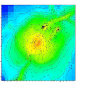
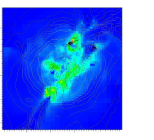
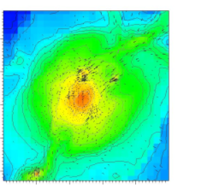
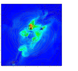
9.2.6 Spatial distribution of turbulent energy

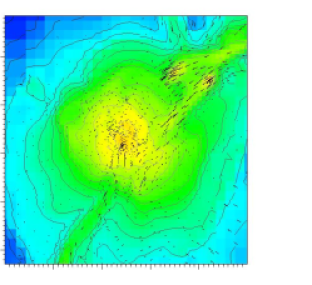
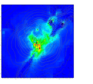
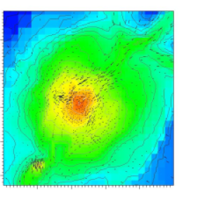
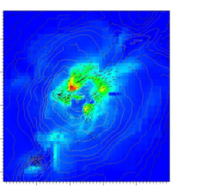
To investigate the time development of the spatial distribution of turbulent energy, we generated slices of density and turbulent energy with the graphical analysis tool VisIt.

The slices are taken around the place of formation of our main galaxy cluster and show a region of size $6.4\times 6.4\,\mathrm{Mpc\ h^{-1}}$ . Overlayed onto the slices are density contour lines and a vector field showing the strength and direction of the velocity. In the density slice at redshift $z=0.15$ (figure a), we can see from the velocity vectors that material is falling onto the cluster along filament from the lower left and from the upper right corner. But from the upper right corner we do not have a smooth inflow of matter, instead two small clumps are approaching. Over the course of the simulation these two clumps merge with the main cluster (figure c-c) and are assimilated completely at redshift $z=0$ . Only the velocity field still shows some disturbance due to the infalling clumps.

In the slice of the turbulent energy (figure b) at $z=0.15$ , we see a hot spot of turbulent energy in the center of our cluster, which is due to a former major merger. The turbulent energy produced due to this merger is declining (figure d-d) and at redshift $z=0$ it is presumably dissipated into internal energy completely, so there is only little turbulent energy left at the center of the cluster.

However the two approaching clumps will drive turbulence again in the cluster. Thereby the left clump can be identified in the turbulent energy slice at $z=0.15$ (figure b) as a ring-like structure, showing that turbulence is not produced in the center of the infalling clump, but is presumably produced at the front (behind a bow shock) and in the wake of the infalling material. But the right clump only shows some turbulence production in its wake, which might be due to its smaller size and smaller velocity. However, on their way towards the main cluster, both clumps develop a hot spot of turbulent energy (figure d-b). The hot spot of turbulent energy can even be identified after the two clumps have merged with the main cluster (figure d) and are not visible in the density slice (figure c) anymore. In this sense, the distribution of turbulent energy traces the local merging history of a galaxy cluster until it is dissipated into heat completely. Also the merging of the two small clumps with the main cluster drives turbulence only in its outer rim, showing that smaller mergers might only be able to drive turbulence in the outer regions ( $r>R_{vir}$ ) of a cluster. But turbulence is sustained for a longer time in a galaxy cluster than one might expect from just looking at density development.

9.2.7 Cluster core analysis

As mentioned we couldn’t use the enzo_anyl tool to compute average values of thermodynamic quantities of the cluster core. Instead we analyzed the cluster core using the interactive parallel visualization and graphical analysis tool VisIt⁴⁹⁴⁹Freely available from https://wci.llnl.gov/codes/visit.. Using this tool we computed several mass-weighted averaged quantities within a sphere of radius $R=0.1\ R_{vir}$ , centered at the cluster center. The results of this analysis are summarized in tables 9.3\subreftab:avg1-9.3\subreftab:avg3.

Run	$m_{bar}$	$\rho$	$T$	$K$	$\sigma$
	$[\mathrm{10^{12}\ M_{\odot}}]$	$[\mathrm{10^{14}\ M_{\odot}\ Mpc^{-3}}]$	$[\mathrm{10^{7}\ K}]$	$[\mathrm{10^{5}\times code\ units}]$	$[\mathrm{km\ s^{-1}}]$
no SGS	2.73	0.996	7.88	4.40	200
SGS	3.37	1.29	6.99	3.38	257

(a) General quantities.

Run	$p_{th}/\rho$	$p_{res}/\rho$	$\frac{p_{res}}{p_{th}+p_{res}}$
	$[\mathrm{10^{16}\ cm^{2}s^{-2}}]$	$[\mathrm{10^{14}\ cm^{2}s^{-2}}]$	$[\mathrm{\%}]$
no SGS	1.05	1.34	1.25
SGS	0.936	2.20	2.30

(b) Resolved and thermal pressure.

Run	$p_{turb}/\rho$	$\epsilon$	$\Sigma$
	$[\mathrm{10^{14}\ cm^{2}s^{-2}}]$	$[\mathrm{10^{-5}\ cm^{2}s^{-3}}]$	$[\mathrm{10^{-5}\ cm^{2}s^{-3}}]$
no SGS	0.0	0.0	0.0
SGS	0.380	3.06	2.92

Table 9.3: Mass weighted values of some quantities, calculated within a sphere with

R=0.1\ R_{vir}

centred at the cluster center at z=0.

The table lists as general quantities of the simulations the baryonic mass $m_{bar}$ inside the chosen sphere, the density $\rho$ , the temperature $T$ , the entropy $K=\frac{T}{\rho^{\gamma-1}}$ with $\gamma=5/3$ and the baryonic velocity dispersion $\sigma=\frac{\sum_{i}m_{i}{\left(v_{i}-\langle v\rangle\right)}^{2}}{m_{bar}}$ at the length scale $l=0.1\ R_{vir}=133\,\mathrm{kpc\ h^{-1}}$ . According to Voit (2005) entropy is the most important quantity to look at, because it determines the structure of the intracluster medium and it records the thermodynamic history of the cluster’s gas; the temperature and density are just manifestations of the entropy. We find that the ratio of the entropies in the cluster core of the two simulations (in the following 1 is used to subscript quantities of the run without SGS model, 2 subscripts quantities of the simulation with SGS model) is

\displaystyle\frac{K_{1}}{K_{2}}=1.30={\left(\frac{\rho_{1}}{\rho_{2}}\right)}% ^{-1}={\left(\frac{\sigma_{1}}{\sigma_{2}}\right)}^{-1}.

(9.19)

Since $\frac{K_{1}}{K_{2}}={\left(\frac{T_{1}}{T_{2}}\right)}{\left(\frac{\rho_{1}}{% \rho_{2}}\right)}^{-2/3}$ by definition, this yields

\displaystyle{\left(\frac{T_{1}}{T_{2}}\right)}={\left(\frac{\rho_{1}}{\rho_{2% }}\right)}^{-1/3}=1.09,

(9.20)

which is roughly fulfilled, since from the data directly we get $T_{1}/T_{2}=1.13$ . So temperature and density are really just manifestations of entropy, but also the velocity dispersion of the baryonic gas in the cluster core seems to be directly connected to the entropy. Because of this, the velocity dispersion at a length scale of $l=0.1\ R_{vir}$ in the simulation with the SGS model is significantely higher than in the simulation without SGS model.

In table b we list the thermodynamic pressure $p_{th}$ and the resolved pressure, which is defined as

\displaystyle p_{res}=\frac{1}{3}\rho\sigma^{2},

(9.21)

and the ratio between resolved and thermodynamic pressure. We see that, in the case of the SGS model simulation, the ratio of resolved to thermal pressure is nearly twice as high compared to the simulation without SGS model, since density and velocity dispersion are higher in the core when using the SGS model.

Listed in table c is also the turbulent pressure, defined as

\displaystyle p_{res}=\frac{1}{3}\rho q^{2},

(9.22)

where $q^{2}$ is related to the velocity fluctuations at grid length scale $l=15.7\,\mathrm{kpc\ h^{-1}}$ . So directly comparing or adding the resolved pressure to the turbulent pressure is not useful, since both are related to the deviations of the velocity on different length scales. However, the ratio of turbulent production $\Sigma$ to turbulent dissipation $\epsilon$ in the core of the cluster is interesting

\displaystyle\frac{\Sigma}{\epsilon}=0.95,

(9.23)

showing that we are actually in a regime of near equilibrium of production and dissipation of turbulent energy, a sign that a turbulent cascade has established.

9.2.8 Influence of SGS parameters on cluster core

In an attempt to better understand the influence of the SGS model on the thermodynamic properties of the cluster core, we conducted a series of simulations with different parameters for the SGS model. Because of our restricted CPU budget we could not afford to do these simulations with the full $128^{3}$ root grid resolution, rather we were only able to do these studies using a root grid resolution of $32^{3}$ grid cells and $32^{3}$ N-body particles. In analogy to the high resolution simulation, we also nested a static child grid inside the root grid, with $32^{3}$ cells and $32^{3}$ N-body particles. The mass of each particle in this grid was $5.8\times 10^{11}\,\mathrm{M_{\odot}\ h^{-1}}$ , so the resolution of the gravitational potential due to dark matter was much lower in these runs. We allowed adaptive grid refinement from level $l=2$ to $l=8$ in a volume of $38.4\,\mathrm{Mpc\ h^{-1}}$ inside this grid, so the effective resolution of the baryonic component and all the other parameters were equal to the high resolution runs. The galaxy clusters that formed in these simulations had a virial mass of roughly $M_{vir}=6.9\times 10^{14}\,\mathrm{M_{\odot}\ h^{-1}}$ and a virial radius of $R_{vir}=1.27\,\mathrm{Mpc\ h^{-1}}$ .

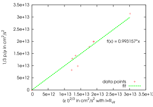
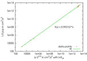
As parameters we chose all combination of $C_{\nu}=(0.0,0.05),C_{\lambda}=(0.0,-0.2),C_{\mathbb{D}}=(0.0,0.4)$ and $C_{p}=(0.0,1.0)$ ⁵⁰⁵⁰Setting $C_{p}=0.0$ means switching off the influence of the turbulent pressure in the momentum equation., which gave use 16 combinations altogether. In complete analogy to the high resolution runs we analyzed the average values of thermodynamic quantities of the cluster core. Albeit one interesting preliminary result emerged. By plotting the average values of the turbulent pressure over the average value of turbulent dissipation in the cluster core (figures a,b), we found that they seem to be related as

\displaystyle\langle\frac{p_{t}(l_{min})}{\rho}\rangle=C(\langle\epsilon% \rangle R_{vir})^{2/3},

(9.24)

where $\langle\rangle$ means the mass weighted average over the cluster core $r<0.1\ R_{vir}$ , $l_{min}=15.6\,\mathrm{kpc\ h^{-1}}$ and $R_{vir}=1.27\,\mathrm{Mpc\ h^{-1}}$ . The constant $C$ can be found from a linear fit to be $C\approx 1$ (see fit in figures a,b). If we use again our scaling relation for the turbulent velocity (9.12), we get with $\langle\frac{p_{t}(l_{min})}{\rho}\rangle=\langle q^{2}(l_{min})\rangle$ and $C=1$

\displaystyle\langle q^{2}(l)\rangle={\left(\frac{R_{vir}}{l_{min}}\right)}^{2% /3}\langle\epsilon\rangle^{2/3}l^{2/3}

(9.25)

If we assume, that the value of $\frac{R_{vir}}{l_{min}}^{2/3}=18.8$ is universal, we get for cluster core turbulence the relation

\displaystyle\langle q^{2}(l)\rangle=18.8\langle\epsilon\rangle^{2/3}l^{2/3}.

(9.26)

In this sense, we can interpret $C_{k,core}=18.8$ as a Kolmogorov constant for the cluster core turbulence, which is more than 10 times higher than what is found for the Kolmogorov constant in simulations of incompressible turbulence.