Adaptively Refined Large-Eddy Simulations of Galaxy Clusters 4 Favre-filtered equations of fluid dynamics 6 AMR and LES

Chapter 5 LES and SGS model

5.1 The concept of LES

The idea behind large eddy simulations (LES) is to solve the filtered equations of fluid dynamics (FE) (4.26) - (4.29) instead of the unfiltered ones (UE) (2.1)-(2.3). There are two reasons for this:

1.

The FE represent a system with a smaller number of resolved degrees of freedom (DOF) compared with the UE. This is a necessary restriction, because the numerical discretization itself acts as a filter²⁰²⁰See section 3.4. and limits the number of DOF which we can resolve in a high Reynolds number flow. In effect this leads to the problem that the outcome of a simulation of turbulence using the UE depends on the numerical scheme used. If instead we solve the FE using a certain subgrid model with a characteristic cutoff length higher than the numerical cutoff length, the outcome of the turbulence simulation is only dependent on our subgrid model and not on the numerical scheme used (Mason and Brown, 1999). From this point of view, we should call a turbulence model simply a filter model.
2.

Using the numerical cutoff as an explicit filter in an energy conserving numerical scheme converts kinetic into internal energy. But the back reaction of the internal energy on the kinetic energy can only be via the pressure term, which is presumably not right. With an explicit turbulence model, we can model the backscattering of small scale fluctuations on the resolved kinetic energy in a much better way (Schmidt, 2004). To model the backscattering we have to know explicitly the amount of energy on the scales between the cutoff scale and the Kolmogorov scale. This is what we call subgrid energy or turbulent energy and that is why the term subgrid scale (SGS) model is appropriate for the unknown terms in the FE.

Unfortunately there is a substantial variety of SGS models in the literature and no agreement on a standard model. An extensive overview of SGS models for incompressible flows can be found for example in the book by Sagaut (2006). There are fewer models explicitly for compressible flows. A simple one, that was first introduced by Schmidt (2004); Schmidt et al. (2006a), will be described in the next sections. This Schmidt model²¹²¹Actually the original implementation of the SGS model proposed by Schmidt et al. (2006a) had severe problems with energy conservation and was notoriously difficult to implement in an AMR code. The version of the Schmidt model described in this work is a simplified version, but it conserves energy and proved to be sufficient for our work., together with some corrections due to Sarkar (1992), which will be outlined later, is the model we use to describe the influence of turbulence on the resolved scales in our work.

5.2 Schmidt model

As we interpret the trace of the generalized central moment of the velocity $\langle\tau\rangle_{ij}$ as a turbulent energy, we can define a velocity of the turbulent motions²²²²This is based on an analogy to kinetic energy in the sense, that $\frac{1}{2}\rho q^{2}=\rho e_{t}$ . $q=\sqrt{2e_{t}}$ , which is used as characteristic velocity of the subgrid terms in the Schmidt model. As a characteristic length scale the size of one grid cell $l_{\Delta}$ is used ²³²³As mentioned, the implicit cutoff of our subgrid = filter model should be greater than the numerical cutoff, so one might object, that $l_{\Delta}$ is too small for that. But every term in the subgrid model is multiplied by some dimensionless constant, which is set to a value high enough to make numerical cutoff effects insignificant..

The Schmidt model neglects the convective flux term $\hat{\tau}(v_{j},e_{int})$ and the gravitational effects $\Gamma$ on the subgrid scales. The models for the other terms are described in the following sections.

5.2.1 Transport term $\mathbb{D}$

The transport or diffusion term is modeled by a gradient hypothesis, by stating that the non-linear term is proportional to the turbulent velocity $q^{2}$ gradient (Kolmogorov-Prandl relation, see Sagaut (2006, p.97))

\displaystyle\mathbb{D}=\frac{\partial}{\partial r_{i}}C_{\mathbb{D}}\langle% \rho\rangle l_{\Delta}q^{2}\frac{\partial}{\partial r_{i}}q.

(5.1)

The constant $C_{\mathbb{D}}$ is calibrated to $C_{\mathbb{D}}\approx 0.4=\frac{2}{5}$ by numerical experiments (Schmidt et al., 2006b).

5.2.2 Pressure dilatation $\lambda$

For $\lambda$ an estimate is used that is presumably only valid in the subsonic (nearly incompressible) regime:

\displaystyle\lambda=C_{\lambda}q^{2}\frac{\partial}{\partial r_{i}}\hat{v}_{i}.

(5.2)

The constant $C_{\lambda}=-\frac{1}{5}$ as found by numerical experiments (Schmidt et al., 2006b).

5.2.3 Turbulent dissipation $\epsilon$

The turbulent dissipation accounts for effects of viscosity on subgrid scales. These effects convert turbulent energy to internal energy even if, on the larger scales, the effect of viscosity can be neglected. The most simple expression which can be built from the characteristic turbulent velocity and length scale for the dissipation is

\displaystyle\epsilon=C_{\epsilon}\frac{q^{3}}{l_{\Delta}}.

(5.3)

For our simulations we will set $C_{\epsilon}=0.5$ .²⁴²⁴Suggested by W. Schmidt, personal communication.

5.2.4 Turbulence production tensor $\hat{\tau}(v_{i},v_{j})$

The turbulence production term is symmetric in its arguments and can therefore be written as follows

\displaystyle\hat{\tau}(v_{i},v_{j})=\hat{\tau}_{ij}=\frac{1}{2}(\hat{\tau}_{% ij}+\hat{\tau}_{ij})=\frac{1}{2}(\hat{\tau}_{ij}+\hat{\tau}_{ji}).

(5.4)

By subtracting the trace of this tensor

\displaystyle\hat{\tau}_{ij}=\frac{1}{2}(\hat{\tau}_{ij}+\hat{\tau}_{ji})-% \frac{1}{n}\delta_{ij}\hat{\tau}_{kk}+\frac{1}{3}\delta_{ij}\hat{\tau}_{kk}

(5.5)

and recognizing that $\hat{\tau}_{kk}=\langle\rho\rangle q^{2}$ we can split the tensor in a symmetric, tracefree part $\hat{\tau}^{*}_{ij}=\frac{1}{2}(\hat{\tau}_{ij}+\hat{\tau}_{ji})-\frac{1}{3}% \delta_{ij}\hat{\tau}_{kk}$ and the trace

\displaystyle\hat{\tau}_{ij}=\hat{\tau}^{*}_{ij}+\frac{1}{3}\delta_{ij}\langle% \rho\rangle q^{2}=\hat{\tau}^{*}_{ij}+p_{t},

(5.6)

where the trace is commonly called turbulent pressure $p_{t}$ .

A model for $\hat{\tau}^{*}_{ij}$ is based on the turbulent viscosity hypothesis. There it is assumed, that $\hat{\tau}^{*}_{ij}$ is of the same form like $S^{*}_{ij}$ for a newtonian fluid, so

\displaystyle\hat{\tau}^{*}_{ij}=-2\eta_{t}S^{*}_{ij}

(5.7)

with a turbulent dynamic viscosity $\eta_{t}=\langle\rho\rangle\nu_{t}=\langle\rho\rangle C_{\nu}l_{\Delta}q$ and

\displaystyle S^{*}_{ij}=\frac{1}{2}{\left(\frac{\partial}{\partial r_{j}}\hat% {v}_{i}+\frac{\partial}{\partial r_{i}}\hat{v}_{j}\right)}-\frac{1}{3}\delta_{% ij}\frac{\partial}{\partial r_{k}}\hat{v}.

(5.8)

The turbulence production term is therefore modeled as

\displaystyle\hat{\tau}(v_{i},v_{j})=-2\langle\rho\rangle C_{\nu}l_{\Delta}qS^% {*}_{ij}+\frac{1}{3}\delta_{ij}\langle\rho\rangle q^{2}.

(5.9)

It should be noted, that in general the old idea of turbulent viscosity (which was first forumlated by Boussinesq (1877)) is incorrect. As Pope (2000) shows, it is only true when the ratio of production of turbulent energy $\Sigma^{*}=\hat{\tau}^{*}_{ij}\frac{\partial v_{i}}{\partial r_{j}}$ to dissipation $\epsilon$ is $\frac{\Sigma^{*}}{\epsilon}\sim 1$ . If this ratio is much greater or much smaller than one the turbulent viscosity hypothesis is incorrect.

Nevertheless since it is the most common idea used to model the turbulent production tensor it is also used in the Schmidt model. Setting the constant $C_{\nu}=0.05$ seems to be a rational choice (Schmidt et al., 2006b).

5.2.5 Summary of the Schmidt model

Using the Schmidt model, the FE form the following system of equations

$\displaystyle\frac{\partial}{\partial t}\langle\rho\rangle+\frac{\partial}{% \partial r_{j}}\hat{v}_{j}\langle\rho\rangle=$	$\displaystyle\ 0,$		(5.10)
$\displaystyle\frac{\partial}{\partial t}\langle\rho\rangle\hat{v}_{i}+\frac{% \partial}{\partial r_{j}}\hat{v}_{j}\langle\rho\rangle\hat{v}_{i}=$	$\displaystyle-\frac{\partial}{\partial r_{i}}(\langle p\rangle+p_{t})+\langle% \rho\rangle\hat{g}_{i}-\frac{\partial}{\partial r_{j}}\hat{\tau}^{*}_{ij},$		(5.11)
$\displaystyle\begin{split}\displaystyle\frac{\partial}{\partial t}\langle\rho% \rangle e_{res}+\frac{\partial}{\partial r_{j}}\hat{v}_{j}\langle\rho\rangle e% _{res}=&\displaystyle-\frac{\partial}{\partial r_{i}}\hat{v}_{i}(\langle p% \rangle+p_{t})+\langle\rho\rangle\hat{v}_{i}\hat{g}_{i}\\ &\displaystyle+\langle\rho\rangle(\lambda+\epsilon)-\hat{v}_{i}\frac{\partial}% {\partial r_{j}}\hat{\tau}^{*}(v_{i},v_{j}),)\end{split}$		(5.12)
$\displaystyle\frac{\partial}{\partial t}\langle\rho\rangle e_{t}+\frac{% \partial}{\partial r_{j}}\hat{v}_{j}\langle\rho\rangle e_{t}=$	$\displaystyle\ \mathbb{D}-\langle\rho\rangle(\lambda+\epsilon)-\hat{\tau}^{*}(% v_{j},v_{i})\frac{\partial}{\partial r_{j}}\hat{v_{i}}-p_{t}\frac{\partial}{% \partial r_{i}}\hat{v_{i}}.$		(5.13)

Again it is often useful to split the equation for resolved energy into an equation for the resolved kinetic energy and internal energy respectively

	$\displaystyle\begin{split}\displaystyle\frac{\partial}{\partial t}\langle\rho% \rangle\hat{e}_{k}+\frac{\partial}{\partial r_{j}}\hat{v}_{j}\langle\rho% \rangle\hat{e}_{k})=&\displaystyle-\hat{v}_{i}\frac{\partial}{\partial r_{i}}(% \langle p\rangle+p_{t})+\langle\rho\rangle\hat{v}_{i}\hat{g}_{i}-\hat{v}_{i}% \frac{\partial}{\partial r_{j}}\hat{\tau}^{*}(v_{i},v_{j}),\end{split}$		(5.14)
	$\displaystyle\begin{split}\displaystyle\frac{\partial}{\partial t}\langle\rho% \rangle\hat{e}_{int}+\frac{\partial}{\partial r_{j}}\hat{v}_{j}\langle\rho% \rangle\hat{e}_{int}=&\displaystyle-(\langle p\rangle+p_{t})\frac{\partial}{% \partial r_{j}}\hat{v}_{j}+\langle\rho\rangle(\lambda+\epsilon).\end{split}$		(5.15)

5.3 Impact of the Schmidt SGS on the fluid equations

5.3.1 General observations

In this section we want to investigate the influence of the Schmidt model on the equations of fluid dynamics. This can be done most easily in a graphical way.

Figure 5.1: Energy transfer in the unfiltered equations of fluid dynamics.

One can see in figure 5.1 the energy transfer between potential, kinetic, and internal energy for the UE. We see that it is possible to convert potential energy into kinetic energy and vice versa, and also kinetic energy into internal energy and vice versa via adiabatic pressure effects. On the other side, irreversible changes of state due to viscous effects can only lead to an increase of internal energy and not(!) vice versa.

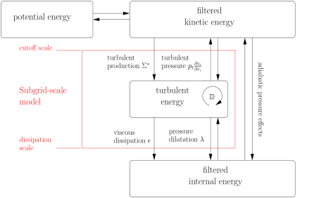
Figure 5.2: Energy transfer in the filtered equations of fluid dynamics with Schmidt SGS.

In figure 5.2 the energy transfer for the FE with the Schmidt model is depicted in the same schematical way. We see that the kinetic energy is now split into two parts: the filtered kinetic energy on resolved scales and the turbulent energy on unresolved scales. From this picture it becomes clear that the turbulent energy is converted to internal energy by the same processes as the filtered kinetic energy. Also it could be converted to potential energy²⁵²⁵Drawing the analogy from the conversion of kinetic into internal energy one might ask if there could be something like irreversible conversion of potential energy into kinetic energy or perhaps vice versa. But from general relativity we know that there is no gravity, there is only curvature of space time. It seems very strange to imagine something like irreversible curvature of space time., but as already mentioned, this effect is neglected in the Schmidt model and therefore not depicted here, as well as the effects due to the convective flux term.

One very important assumption that has not yet been discussed, but is also depicted in figure 5.2, is that conversion of resolved kinetic energy into internal energy due to viscous effects is neglected. Basically all SGS models that make use of the turbulent viscosity hypothesis, and therefore also the Schmidt model, assume that for high Reynolds numbers the turbulent viscosity is much greater than the real viscosity. Why this assumption can be made will be explained in section 5.3.2.

The last conclusion that can be drawn from this pictures is that certain quantities are related to the cutoff scale ( $\Sigma^{*},p_{t}$ ) and others are related to the dissipation scale ( $\epsilon$ , $\lambda$ ). Nevertheless we find that the turbulent dissipation $\epsilon$ in the Schmidt model (and also in most other SGS models) is modeled depending on the cutoff scale $l_{\Delta}$ , although it should ultimately only depend on the dissipation scale. As we shall see later this is a point of major concern in the development of a SGS model for an adaptive grid code.

5.3.2 Dimensional analysis

In complete analogy to the UE²⁶²⁶See appendix A. we can do a dimensionless analysis for the FE with the Schmidt model.

Momentum equation

Introducing the dimensionless quantities

\displaystyle e_{t}^{*}=\frac{e_{t}}{q^{2}_{0}},\ p_{t}^{*}=\frac{p_{t}}{\rho_% {0}q^{2}_{0}},\ \tau_{ij}^{**}=\frac{\tau_{ij}}{\eta v_{0}/l_{0}}=\frac{\tau_{% ij}}{\rho_{0}q_{0}v_{0}}

(5.16)

the momentum equation can be written as

	$\displaystyle\frac{l_{0}}{t_{0}v_{0}}\frac{\partial}{\partial t^{}}\langle% \rho^{}\rangle\hat{v}^{}_{i}+\frac{\partial}{\partial r_{j}^{}}\hat{v}^{}_% {j}\langle\rho^{}\rangle\hat{v}^{*}_{i}=$	$\displaystyle+\frac{\rho_{0}g_{0}l_{0}}{\rho_{0}v_{0}^{2}}\langle\rho^{}% \rangle\hat{g^{}}_{i}-\frac{p_{0}}{\rho_{0}v_{0}^{2}}\frac{\partial}{\partial r% ^{}_{i}}\langle p^{}\rangle-\frac{q_{0}^{2}}{v_{0}^{2}}\frac{\partial}{% \partial r^{*}_{i}}p_{t}$		(5.17)
		$\displaystyle+\frac{\eta_{0}}{\rho_{0}l_{0}v_{0}}\frac{\partial}{\partial r_{j% }^{}}\langle\sigma^{{}^{\prime}}_{ij}\rangle-\frac{q_{0}}{v_{0}}\frac{% \partial}{\partial r^{}_{j}}\hat{\tau}^{*}_{ij}$		(5.18)

From this we can estimate, that the turbulent pressure will become important, when

\displaystyle\frac{q_{0}^{2}}{v_{0}^{2}}\geq\frac{p_{0}}{\rho_{0}v_{0}^{2}}% \Rightarrow\frac{q_{0}^{2}}{p_{0}/\rho_{0}}\geq 1

(5.19)

If we now introduce the turbulent Mach number

\displaystyle M_{t}=\frac{q_{0}}{c_{s}}

(5.20)

and use $\frac{p_{0}}{\rho_{0}}=\frac{c_{s}^{2}}{\gamma}$ we see that the turbulent pressure will dominate over the thermal pressure, if

\displaystyle M_{t}^{2}\geq\gamma.

(5.21)

The turbulence production tensor $\hat{\tau}^{*}_{ij}$ becomes important compared to the stress tensor, if

\displaystyle\rho_{0}q_{0}l_{0}\geq\eta_{0}.

(5.22)

So we see that if the turbulent viscosity is greater than the physical viscosity the turbulent production tensor will dominate over the stress tensor in the FE. The physical viscosity is

\displaystyle\eta_{0}\sim\rho_{0}\sqrt{u_{0}}l_{\lambda}

(5.23)

where $u_{0}$ is the mean thermal energy and $l_{\lambda}$ the mean free path of a particle, so we see that the turbulent viscosity is greater than the physical viscosity, if

\displaystyle\frac{q_{0}^{2}}{u_{0}}\geq{\left(\frac{l_{\lambda}}{l_{0}}\right% )}^{2}\Rightarrow\frac{q_{0}^{2}}{u_{0}}\geq{\left(Kn\right)}^{2},

(5.24)

which means the ratio of turbulent energy to internal energy must be greater than the square of the Knudsen number $Kn=\frac{l_{\lambda}}{l_{0}}$ . Since in any case the Knudsen number must be much smaller than one for the continuum approximation to hold, we can practically always assume that the turbulent production tensor will dominate over the stress tensor.²⁷²⁷Of course this analysis is restricted to $l_{0}>l_{k}$ , since if we resolve the fluid up to the Kolmogorov length $l_{k}$ the turbulent energy will be zero. For scales smaller than the Kolmogorov length we cannot neglect the influence of the physical viscosity. This justifies our assumption in the Schmidt model to neglect the influence of the stress tensor completely in the momentum equation and therefore also in the kinetic energy equation.

For completeness we also compare the gravitational force to the turbulent pressure, which yields

\displaystyle\frac{\rho_{0}q_{0}^{2}}{\rho_{0}g_{0}l_{0}}\geq 1.

(5.25)

Turbulence will thus dominate over gravity in the momentum equation, if the average turbulent energy is greater than the gravitational energy.

Internal energy equation

The internal energy equation can be analyzed in the same way as the momentum equation using the additional dimensionless quantities

\displaystyle e_{int}^{*}=\frac{e_{int}}{u_{0}},\ \lambda^{*}=\frac{\lambda}{% \lambda_{0}}=\frac{\lambda}{q_{0}^{2}v_{0}/l_{0}},\ \epsilon^{*}=\frac{% \epsilon}{\epsilon_{0}}=\frac{\epsilon}{q_{0}^{3}/l_{0}}.

(5.26)

This results in

\displaystyle\begin{split}\displaystyle\frac{l_{0}}{t_{0}u_{0}}\frac{\partial}% {\partial t^{*}}\langle\rho^{*}\rangle\hat{e}_{int}^{*}+\frac{\partial}{% \partial r_{j}^{*}}\hat{v}_{j}^{*}\langle\rho^{*}\rangle\hat{e}_{int}^{*}=&% \displaystyle-\frac{p_{0}}{\rho_{0}v_{0}^{2}}\langle p^{*}\rangle\frac{% \partial}{\partial r_{j}^{*}}\hat{v}_{j}^{*}+\frac{\eta_{0}v_{0}}{\rho_{0}u_{0% }l_{0}}\langle\sigma^{{}^{\prime}*}\rangle\frac{\partial}{\partial r_{j}^{*}}% \hat{v}_{j}^{*}\\ &\displaystyle-\frac{q_{0}^{2}}{u_{0}}p_{t}\frac{\partial}{\partial r_{j}^{*}}% \hat{v}_{j}^{*}+\frac{q_{0}^{2}}{u_{0}}\langle\rho^{*}\rangle\lambda^{*}+\frac% {q_{0}^{3}}{v_{0}u_{0}}\langle\rho^{*}\rangle\epsilon^{*}.\end{split}

(5.27)

We see that the pressure dilatation $\lambda$ will dominate over the pressure term if

\displaystyle M_{t}^{2}\geq\gamma

(5.28)

and that the turbulent dissipation $\epsilon$ will dominate over the viscous dissipation, if

\displaystyle\rho_{0}l_{0}q_{0}{\left(\frac{q_{0}}{v_{0}}\right)}^{2}\geq\eta_% {0}\Rightarrow{\left(\frac{q_{0}}{v_{0}}\right)}^{2}\geq\frac{\eta_{0}}{\eta_{% t}}.

(5.29)

As shown in section 5.3.2 $\eta_{0}\ll\eta_{t}$ , so we can always neglect the influence of the stress tensor in the internal energy equation. This also leads to the conclusion, that turbulence will be the only source of entropy in the equations, since the only irreversible conversion of energy into internal energy is via turbulent dissipation $\epsilon$ .

Turbulent energy equation

For the dimensional analysis of the turbulent energy equation we need the additional dimensionless quantity

\displaystyle\mathbb{D}^{*}=\frac{\mathbb{D}}{\rho_{0}q_{0}^{3}/l_{0}}.

(5.30)

Inserting it together with the dimensionless quantities introduced in the former sections yields

\displaystyle\frac{l_{0}}{t_{0}u_{0}}\frac{\partial}{\partial t^{*}}\langle% \rho^{*}\rangle e_{t}^{*}+\frac{\partial}{\partial r_{j}^{*}}\hat{v}_{j}^{*}% \langle\rho^{*}\rangle e_{t}^{*}=

\displaystyle\ \frac{q_{0}}{v_{0}}{\left(\mathbb{D}^{*}-\langle\rho^{*}\rangle% \epsilon^{*}\right)}-\frac{v_{0}}{q_{0}}\hat{\tau}^{**}_{ji}\frac{\partial}{% \partial r_{j}^{*}}\hat{v_{i}^{*}}-p_{t}^{*}\frac{\partial}{\partial r_{i}^{*}% }\hat{v_{i}^{*}}-\langle\rho^{*}\rangle\lambda^{*}.

(5.31)

This analysis shows that the behavior of turbulent energy equation can be completely characterized by the ratio $\frac{q_{0}}{v_{0}}$ . If $\frac{q_{0}}{v_{0}}\gg 1$ , then only diffusion $\mathbb{D}$ and dissipation $\epsilon$ are relevant. If $\frac{q_{0}}{v_{0}}\ll 1$ then the equation is dominated by the turbulent production term $\Sigma^{*}=\hat{\tau}^{*}_{ji}\frac{\partial}{\partial r_{j}}\hat{v_{i}}$ and only if $\frac{q_{0}}{v_{0}}\approx 1$ do all terms contribute to the equation.

5.4 Sarkar model

The effect of compressibility on the structure of turbulence is an important but difficult topic in turbulence modeling and is not really taken into account by the Schmidt model. Sarkar (1992) performed simulations of simple compressible flows and investigated the influence of the mean Mach number of the flow on the turbulent dissipation $\epsilon$ and the pressure dilatation $\lambda$ . Based on this analysis he suggested different models for these terms, which we will describe in the following sections. These modifications have been proven to yield good results²⁸²⁸See Shyy and Krishnamurty (1997). and that’s why we use them in the course of this work, when we reach the limitations of the original Schmidt model with our simulations.

5.4.1 Turbulent dissipation $\epsilon$

As a major effect of compressibility from direct numerical simulation Sarkar (1992) identifies that the growth rate of kinetic energy decreases when the initial turbulent Mach number increases. This means that the dissipation of kinetic energy (and therefore also for the turbulent energy) increases with the turbulent Mach number $M_{t}$ and Sarkar (1992) suggests accounting for this effect by using

\displaystyle\epsilon=C_{\epsilon}\frac{q^{3}}{l_{\Delta}}(1+\alpha_{1}M_{t}^{% 2})

(5.32)

with $\alpha_{1}=0.5$ as a model for the dissipation of turbulent energy.

5.4.2 Pressure dilatation $\lambda$

Based on a decomposition of all variables of the equation for instantaneous pressure²⁹²⁹For a derivation see appendix E.

\displaystyle\frac{\partial^{2}}{\partial r_{i}^{2}}p=\frac{\partial^{2}}{% \partial t^{2}}\rho-\frac{\partial^{2}}{\partial r_{i}\partial r_{j}}(\rho v_{% i}v_{j}-\sigma^{\prime}_{ij})

(5.33)

into a mean and a fluctuating part and comparisons with direct numerical simulations of simple compressible flows Sarkar (1992) proposed a different model for the pressure dilatation

\displaystyle\lambda=\alpha_{2}M_{t}\hat{\tau}^{*}_{ij}\frac{\partial\hat{v}_{% i}}{\partial r_{j}}-\alpha_{3}M_{t}^{2}C_{\epsilon}\frac{q^{3}}{l_{\Delta}}-8% \alpha_{4}M_{t}^{2}p_{t}\frac{\partial\hat{v}_{k}}{\partial r_{k}}

(5.34)

with $\alpha_{2}=0.15$ , $\alpha_{3}=0.2$ obtained from a curve fit of the model with DNS simulation. Unfortunately Sarkar (1992) does not specify a value for $\alpha_{4}$ , so there is some confusion in the literature about it. For example Shyy and Krishnamurty (1997) set $\alpha_{4}=0$ and still found the Sarkar model in good agreement with their DNS simulation. In this work, we adopt a value of $\alpha_{4}=\alpha_{2}^{2}/2$ , which was suggested in a work by Schmidt (2007).

	$\displaystyle\frac{l_{0}}{t_{0}v_{0}}\frac{\partial}{\partial t^{}}\langle% \rho^{}\rangle\hat{v}^{}_{i}+\frac{\partial}{\partial r_{j}^{}}\hat{v}^{}_% {j}\langle\rho^{}\rangle\hat{v}^{*}_{i}=$	$\displaystyle+\frac{\rho_{0}g_{0}l_{0}}{\rho_{0}v_{0}^{2}}\langle\rho^{}% \rangle\hat{g^{}}_{i}-\frac{p_{0}}{\rho_{0}v_{0}^{2}}\frac{\partial}{\partial r% ^{}_{i}}\langle p^{}\rangle-\frac{q_{0}^{2}}{v_{0}^{2}}\frac{\partial}{% \partial r^{*}_{i}}p_{t}$		(5.17)
		$\displaystyle+\frac{\eta_{0}}{\rho_{0}l_{0}v_{0}}\frac{\partial}{\partial r_{j% }^{}}\langle\sigma^{{}^{\prime}}_{ij}\rangle-\frac{q_{0}}{v_{0}}\frac{% \partial}{\partial r^{}_{j}}\hat{\tau}^{*}_{ij}$		(5.18)