Adaptively Refined Large-Eddy Simulations of Galaxy Clusters 1 Introduction 3 Filter formalism

Chapter 2 Turbulence

The equations for a general compressible, viscous, selfgravitating fluid with density $\rho(r_{i},t)$ , momentum density $\rho v_{i}(r_{i},t)$ and total energy density $\rho e(r_{i},t)$ are²²see eg. Landau and Lifschitz (1991).

$\displaystyle\frac{\partial}{\partial t}\rho+\frac{\partial}{\partial r_{j}}(v% _{j}\rho)$	$\displaystyle=0,$	(2.1)
$\displaystyle\frac{\partial}{\partial t}(\rho v_{i})+\frac{\partial}{\partial r% _{j}}(v_{j}\rho v_{i})$	$\displaystyle=-\frac{\partial}{\partial r_{i}}p+\frac{\partial}{\partial r_{j}% }\sigma^{\prime}_{ij}+\rho g_{i},$	(2.2)
$\displaystyle\frac{\partial}{\partial t}(\rho e)+\frac{\partial}{\partial r_{j% }}(v_{j}\rho e)$	$\displaystyle=-\frac{\partial}{\partial r_{j}}(v_{j}p)+\frac{\partial}{% \partial r_{j}}(v_{i}\sigma^{\prime}_{ij})+v_{i}\rho g_{i},$	(2.3)

with Newtonian gravity (Poisson Equation)

\displaystyle\frac{\partial}{\partial r_{j}}g_{j}=4\pi G\rho

(2.4)

and an equation of state to compute the pressure $p(r_{i},t)$ dependent on the material of the fluid. For a Newtonian fluid the stress tensor $\sigma_{ij}$ is of the form³³For a derivation see Appendix C.

\displaystyle\sigma^{\prime}_{ij}=2\eta{\left[\frac{1}{2}{\left(\frac{\partial v% _{i}}{\partial r_{j}}+\frac{\partial v_{j}}{\partial r_{i}}\right)}-\frac{1}{3% }\delta_{ij}\frac{\partial v_{k}}{\partial r_{k}}\right]}+\zeta\delta_{ij}% \frac{\partial v_{k}}{\partial r_{k}},

(2.5)

where the so called dynamic viscosity $\eta$ and the second viscosity $\zeta$ are defined to be constants⁴⁴The literature on incompressible flows often defines the so called kinematic viscosity $\nu=\frac{\eta}{\rho}$ . It should be noted, that this quantity is a constant only for fluids of constant density and cannot be used in a meaningful way when discussing compressible flows. in a Newtonian fluid.

This system of differential equations is complex and highly nonlinear if the nonlinear advection term $\frac{\partial}{\partial r_{j}}(v_{j}\rho v_{i})$ dominates in the momentum equation (2.2) and in general can be solved only numerically. The influence of the advection term can be estimated by writing down the momentum equation in dimensionless form, which yields⁵⁵See Appendix A.

\displaystyle\underbrace{\frac{l_{0}}{v_{0}t_{0}}}_{Sr}\frac{\partial}{% \partial t^{*}}(\rho^{*}v_{i}^{*})+\frac{\partial}{\partial r_{j}^{*}}(v_{j}^{% *}\rho^{*}v_{i}^{*})

\displaystyle=-\underbrace{\frac{p_{0}}{\rho_{0}v_{0}^{2}}}_{Ma^{-2}_{iso}}% \frac{\partial}{\partial r_{i}^{*}}p^{*}+\underbrace{\frac{\sigma_{0}}{\rho_{0% }v_{0}^{2}}}_{Re^{-1}}\frac{\partial}{\partial r_{j}^{*}}\sigma_{ij}^{*}+% \underbrace{\frac{\rho_{0}g_{0}l_{0}}{\rho_{0}v_{0}^{2}}}_{Fr^{-1}}\rho^{*}g_{% i}^{*}.

(2.6)

The arising dimensionless numbers⁶⁶The Strouhal number $S r$ can be set to one by assuming $v_{0}=\frac{l_{0}}{t_{0}}$ . ( $R e$ = Reynolds number, $Ma_{iso}$ = isothermal Mach number, and $F r$ = Froude number) show the ratio of the mean pressure energy density $p_{0}$ , the mean potential energy density $\rho_{0}g_{0}l_{0}$ , and the mean energy dissipation density $\sigma_{0}$ to the mean kinetic energy density $\rho_{0}v_{0}^{2}$ . If all these numbers are much greater than one (which means the mean kinetic energy is big compared to the other energies), the advection term dominates and the fluid flow is called turbulent.

2.1 Phenomenology of Turbulence

As there is no accepted theory of compressible, selfgravitating turbulence we have to restrict the following discussion to incompressible turbulence. For an incompressible fluid, it can be shown that the Reynolds number

\displaystyle Re=\frac{\rho_{0}v_{0}^{2}}{\sigma_{0}}=\frac{\rho_{0}l_{0}v_{0}% }{\eta_{0}}

(2.7)

is the only number which characterizes the dynamics of the fluid flow (Feynman, 1964).

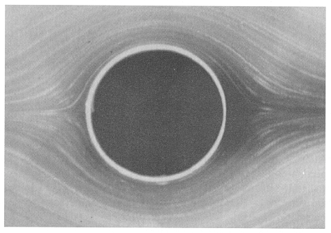
Figure 2.1: Laminar flow past a cylinder at $Re=0.16$ (Frisch, 1995).

If the Reynolds numbers is small, which is the case for high viscosity and/or low flow speed, we call the fluid laminar. In this laminar state the streamlines of the fluid exhibit all the symmetries of the equations and boundary conditions. This can be seen in figure 2.1, where the streamlines of a fluid around a cylinder show up-down and left-right symmetry.⁷⁷ Actually the streamlines also show z-invariance (along the axes of the cylinder) and time-invariance, but they do not show cylindrical symmetry as the direction of the fluid flow breaks this symmetry.

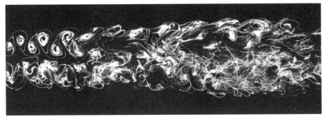
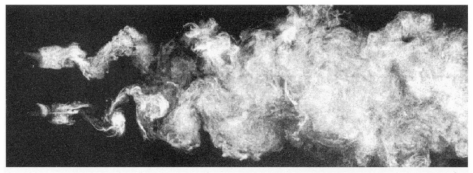
With increasing Reynolds number, the left-right symmetry first (figure a) and then the up-down symmetry are broken (figure b). If $Re>1000$ , the flow becomes completely chaotic and all symmetries are broken. Nevertheless, looking at the flow at smaller scales $l$ far from the boundaries, all the symmetries of the equations seem to be restored in a statistical sense. This state of flow is called fully developed turbulence.

However at the smallest scales of the flow $l_{k}$ , the flow will “behave” laminar again. This means that the Reynolds number becomes smaller on smaller scales and implies that the Reynolds number is scale dependent

\displaystyle Re(l)=\frac{\rho v(l)l}{\eta}.

(2.8)

How the Reynolds number depends on the scales of the flow is explained by the Kolmogorov theory of incompressible turbulence.

2.2 The Kolmogorov theory

Kolmogorov first described his theory of turbulence in 1941. Here we discuss the modern formulation of the Kolmogorov theory as explained in Frisch (1995) and Pope (2000).

According to Frisch, Kolmogorovs theory is based on three assumptions which are valid in the limit of infinite Reynolds numbers, at small scales $l$ $(l_{k}\ll l\ll l_{0})$ and away from boundaries:

1.

All the possible symmetries of the Navier-Stokes equation, usually broken by the mechanisms producing the turbulent flow, are restored in a statistical sense.
2.

The turbulent flow is self-similar.
3.

The turbulent flow has a finite nonvanishing mean rate of dissipation $\langle\epsilon\rangle$ per unit mass.

The mean rate of dissipation is defined as the mean rate of change of kinetic energy

\displaystyle\langle\epsilon\rangle=\langle\frac{d}{dt}e_{kin}\rangle\sim\frac% {v_{0}^{2}}{l_{0}/v_{0}}=\frac{v_{0}^{3}}{l_{0}}=const.

(2.9)

Using this Kolmogorov derived, that for homogeneous and isotropic incompressible turbulence the third order structure function⁸⁸For a definition of structure functions see appendix D.4. $S_{3}(v(l))$ is equal to the mean rate of dissipation times minus four-fifths the length scale $l$ of the structure function

\displaystyle S_{3}(v(l))=-\frac{4}{5}\langle\epsilon\rangle l.

(2.10)

This is the famous four-fifths law of Kolmogorov. From it and the self similarity assumption, Kolmogorov deduces that the structure functions of order $p$ scale like

\displaystyle S_{p}(v(l))\sim\langle\epsilon\rangle^{p/3}l^{p/3}.

(2.11)

Because the second order structure function can be expressed as Fourier transform of the longitudinal velocity spectrum⁹⁹Also see appendix D.4. $\left\lvert V_{\parallel}(k)\right\rvert^{2}\sim e_{kin}(k)$ and the wave numbers $k$ are related to length scales $l$ via $k\sim l^{-1}$ it follows for the specific kinetic energy in Fourier space

\displaystyle e_{kin}(k)\sim\langle\epsilon\rangle^{2/3}k^{-2/3}.

(2.12)

The energy spectrum $E(k)$ is the kinetic energy in the wave number interval between $k$ and $k+dk$ , which is then

\displaystyle E(k)\sim\frac{d}{dk}e_{kin}(k)=C_{k}\langle\epsilon\rangle^{2/3}% k^{-5/3}.

(2.13)

This is the celebrated result of Kolmogorovs theory of incompressible turbulence. The constant $C_{k}$ is therefore called the Kolmogorov constant and is experimentally and numerically found to be $C_{k}\approx 1.6$ (Yokokawa et al., 2002).

It should be noted that the rate of dissipation $\langle\epsilon\rangle$ is not the rate of conversion of kinetic energy into internal energy, rather it describes the amount of energy which is transfered from the bigger to the smaller scales, without the influence of viscosity. The kinetic energy is converted to internal energy only on scales smaller than the Kolmogorov scale $l_{k}$ , where the Reynolds number becomes unity. From this and the relation $S_{1}(v(l))\sim v(l)\sim\langle\epsilon\rangle^{1/3}l^{1/3}$ we can derive an expression for the Kolmogorov scale

\displaystyle Re(l_{k})=1=\frac{\rho v_{l_{k}}l_{k}}{\eta}=\frac{\langle% \epsilon\rangle^{1/3}l_{k}^{4/3}}{\nu}\Rightarrow l_{k}={\left(\frac{\nu^{3}}{% \langle\epsilon\rangle}\right)}^{1/4}.

(2.14)

Using the definition of the dissipation (2.9) in (2.14), we obtain for the ratio between the largest integral length $l_{0}$ and the Kolmogorov length $l_{k}$

\displaystyle\frac{l_{0}}{l_{k}}={\left(\frac{\nu^{3}}{l_{0}^{3}v_{0}^{3}}% \right)}^{-1/4}=Re^{3/4}.

(2.15)

We can use this to estimate the number of degrees of freedom of a three-dimensional fluid flow at a point of time

\displaystyle N_{f}={\left(\frac{l_{0}}{l_{k}}\right)}^{3}=Re^{9/4}.

(2.16)

One consequence of this is that the storage requirement of a fully resolved numerical simulation grows as $Re^{9/4}$ . ¹⁰¹⁰ Using this to estimate the Reynolds number from the biggest direct numerical simulation today by Yokokawa et al. (2002) on the Earth simulator with a resolution of $4096^{3}$ grid cells yields $Re\approx 65536$ . Since the time step must usually be taken proportional to the spatial mesh, the total number of operations to integrate the equations for a fixed number of dynamical times is

\displaystyle N={\left(\frac{l_{0}}{l_{k}}\right)}^{4}=Re^{3}.

(2.17)

As the typical Reynolds numbers in astrophysical context are of the order of $10^{8}$ (Kritsuk et al., 2007) up to $10^{14}$ (Schmidt et al., 2006b) we would need a computer with at least $10^{18}$ Bytes (1 Exabyte) of memory and $10^{16}$ FLOPS¹¹¹¹Floating point operations per second. (10 PetaFLOPS) running for a year to resolve fully an astrophysical simulation. And even if we could efficiently make use of the fact, that turbulence is not volume filling at a point of time, it remains intractable to resolve completely the turbulent fluid dynamics encountered in astrophysics (Schmidt et al., 2006b).

Therefore we can only treat explicitly a limited number of degrees of freedom, which correspond to the largest scales of the system. The influence of the turbulent dynamics from smaller scales onto larger scales has to be treated in a statistical way. How the dynamics on small scales and the dynamics on large scales are interconnected, can be seen by explicitly filtering the equations of fluid dynamics.