Chapter 6 AMR and LES

The most powerful technique for grid-based solvers to resolve localized and anisotropic structures in a flow is adaptive mesh refinement (AMR). Using AMR the grid will be refined³⁰³⁰Refined means that the values from a coarse parent grid are interpolated onto a finer child grid and then integrated independently from the coarse grid. However, the way how to interpolate the values from coarse to fine grid is not discussed in the literature and most often not described by the developers of AMR fluid codes. Although outside the scope of our work, the dependence of the solution and the spectrum of the solution on this interpolation routines should be investigated in the future., depending on a refinement criterion, only at the defined “interesting” areas of the flow field. This allows for treating a much bigger range of dynamic scales of the fluid with the same number of grid cells compared to a static grid.

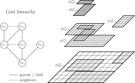
The grid structure can thereby be understood as a hierarchy of grid patches (see figure 6.1) that approximate the flow on various levels of resolution (Berger and Oliger, 1984; Berger and Colella, 1989). But not only the spatial resolution, also the time resolution is adaptive. All grids on a given level are advanced simultaneously with a maximum timestep such that the Courant condition is satisfied by all the cells on that level. This results in a hierarchy of timesteps: a coarse, parent grid on level $l$ is advanced by $\mathrm{\Delta }{t}^{\text{coarse}}$, and then its finer, subgrid(s) on level $l+1$ are advanced by one or more timesteps $\mathrm{\Delta }{t}^{\text{fine}}$ until they reach the same physical time as their parent grid. At this point, the coarse grid values $u^{\text{coarse}}$ are replaced by the underlying fine grid values $u_i^{\text{fine}}$ using mass weighted, conservative averaging³¹³¹Density itself is not weighted by mass but only by volume ${\rho }^{\text{coarse}}=\frac{1}{V}{\sum }_i{\rho }_i^{\text{fine}}{V}_i$.

$u^{\text{coarse}}={\displaystyle \frac{1}{M}}{\displaystyle \sum _i}{\rho }_i{u}_i^{\text{fine}}{V}_i,$

(6.1)

where $M={\sum }_i{\rho }_i{V}_i$ is the total mass of the underlying subgrid cells and $V_i$ is the volume of a fine grid cell.

To completely ensure mass conservation, however, one not only has to replace the coarse grid values with averaged fine grid values, but also must correct coarse grid cells, which abut fine grid cells, but are not themselves covered by any fine grid. This can be understood, by writing the underlying, conservative, explicit finite difference scheme as

$u_n(t+\mathrm{\Delta }{t}^{\text{coarse}})=u(t)-{\displaystyle \frac{\mathrm{\Delta }{t}^{\text{coarse}}}{\delta x}}\left(F_{n+1/2}^{\text{coarse}}-F_{n-1/2}^{\text{coarse}}\right),$

(6.2)

where $F_{n\pm 1/2}$ are the fluxes on the left and right hand side of the cell number $n$ respectively. If the left hand side of cell $n$ abuts on a fine grid, the flux $F_{n-1/2}^{\text{coarse}}$ has to be replaced by the fluxes of the neighboring fine grid cells

$F_{n-1/2}^{\text{fine}}={\displaystyle \sum _i}{F}_{i+1/2}(t+i\mathrm{\Delta }{t}^{\text{fine}}),$

(6.3)

where the sum is due to the refinement in time. This flux replacement is most often implemented as a correction pass after a grid has been integrated using equation 6.2

$u_n(t+\mathrm{\Delta }{t}^{\text{coarse,corr}})=u_n(t+\mathrm{\Delta }{t}^{\text{coarse}})+\mathrm{\Delta }F$

(6.4)

with

$\mathrm{\Delta }F=-F_{n-1/2}^{\text{coarse}}+{\displaystyle \sum _i}{F}_{i+1/2}(t+i\mathrm{\Delta }{t}^{\text{fine}}).$

(6.5)

This ”Flux Correction” step is the most difficult and error-prone part of an AMR implementation, since one has to track all the fluxes of the time varying boundaries of coarse and fine grids, and correctly maintain them between processors, if the simulation is run in parallel on several CPUs.

Nevertheless, if done correctly, this technique has proven to be very well suited for astrophysical problems which include strong shocks or gravitational collapse (Bryan et al., 2001) among many other applications. However, in the case of astrophysically relevant Reynolds numbers³²³²See section 2.2. even with AMR we cannot hope to resolve all relevant scales down to the dissipative scales (Schmidt et al., 2006a).

But as mentioned in the introduction, we do not have to resolve all scales if we use a SGS model. We only need to resolve energy-containing motions. That’s the reason why combining LES and AMR offers the possibility of treating turbulence in astrophysical simulations in a much better way. Though there is one big problem, when trying to combine LES with AMR. Most of the terms of a SGS model like the Schmidt model do depend on the cutoff scale $l_{\mathrm{\Delta }}$ of the grid and this cutoff scale varies in time and space if one uses AMR. But when filtering the fluid dynamic equations, we assumed our filter operation to commute with time and spatial derivatives and hence be static and isotropic, in direct contradiction to the methods of AMR. Therefore combining LES and AMR seem to pose a big challenge and only few attempts have been made so far.

Although proposals to combine LES and AMR are frequently made (e.g Pope (2004)), literature on the topic is still rare.

Probably the first attempt to combine LES and AMR is due to Sullivan et al. (1996). They used a kind of zero-filling to interpolate the solution between the coarse and fine grid. But their simulation of planetary boundary layers only used one static nested fine grid within a coarse grid and was therefore of limited use for more general problems. Boersma et al. (1997) came to the conclusion, using the methods of Sullivan et al. (1996), that with respect to statistics, the nested grid simulations are clearly superior to the results obtained with a simulation on a coarse grid in the whole flow domain. They also found that their solution of a 2d Kelvin-Helmholtz instability improves even in the area only covered by the coarse grid, an encouraging fact. Another approach to large eddy simulations using AMR was put forward by Cook (1999). He presented a method for computing a fine grid solution given a coarse grid solution and vice versa using a deconvolution with a gaussian filter. He showed how to avoid commutation errors with this technique, and that boundary errors are usually small. He also emphasized the advantage of using several nested grids instead of one stretched grid. He came to the conclusion, however, that shocks and other high-frequency phenomena should not be allowed to cross grid boundaries, which renders his method invalid for simulating compressible flows in astrophysics.

A sophisticated approach is the multilevel algorithm for large-eddy simulation of turbulent flow by Terracol et al. (2001, 2003). ³³³³Also see the book of Sagaut et al. (2006). But although they use a time-dependent number of grids, the finer grids in their simulations always cover the whole computational domain and and are only used to improve the overall LES performance. Also methods based on wavelets have been proposed by Goldstein and Vasilyev (2004) and Léonard et al. (2006) and even for adaptive, unstructured grids (Mitran, 2001; Nägele and Wittum, 2003), but seem to be rarely used. The newest method to combine LES and blockstructured AMR comes from Pantano et al. (2007), but they use a very different SGS-model compared to the Schmidt model considered in our work and therefore it is unclear if their method is of general use.

Finally in an astrophysical context Falle (1994) claims to use a $k$-$ϵ$ subgrid scale model build into the hierarchical adaptive grid code $\mu$Cobra to treat the effect of turbulence on the large structure of radio jets. However the specific problems due to adaptive gridding are not mentioned in this paper and Falle (1994) himself comes to the conclusion that his treatment of turbulence is rather dubious. Nevertheless, the same model seems to be used in a recent paper by Pope et al. (2008) on the generation of optical emission-line filaments in galaxy clusters.

In this chapter, we want to present a new simple method to address the problem of combination of AMR and LES. It is based on the finding of section 5.3, that the turbulent dissipation $ϵ$ is related to the dissipation scale, but in the Schmidt model (and most other SGS models) modeled depending on the cutoff scale. This is no problem, if we use a static grid in our fluid dynamic simulation, but it poses a problem in AMR simulations. The reason is that the time and spatial variance of $l_{\mathrm{\Delta }}$ in an adaptive simulation leads to an artificial dependence of $ϵ$ on the grid structure of the simulation. But as we now from Kolmogorovs theory of turbulence the average rate of dissipation should be independent of the length scale in fully developed turbulence. This would not be the case in a AMR simulation of fully developed turbulence, if $ϵ$ depends on the cutoff scale, since the average turbulent energy and therefore the turbulent velocity $q$ is independent of the lengthscale in a conservative AMR code. So our idea is to try to enforce the independence of $ϵ$ on the grid patches of different cutoff scale in our AMR simulations of turbulence. Explicitely this can be written as

$ϵ(l_{\mathrm{\Delta },1})=ϵ(l_{\mathrm{\Delta },2}),l_{\mathrm{\Delta },1}>l_{\mathrm{\Delta },2}$

(6.6)

where $ϵ(l_{\mathrm{\Delta },1})$ is the value of the turbulent dissipation in one grid cell of the coarse grid and $ϵ(l_{\mathrm{\Delta },2})$ is the average value of the turbulent dissipation after interpolation on a overlapping fine grid patch. Inserting our model for epsilon (5.3) we get

$C_{ϵ,1}{\displaystyle \frac{q_1^3}{l_{\mathrm{\Delta },1}}}=C_{ϵ,2}{\displaystyle \frac{q_2^3}{l_{\mathrm{\Delta },2}}}.$

(6.7)

Assuming $C_{ϵ,1}=C_{ϵ,2}$ this leads to

${\displaystyle \frac{q_1^2}{q_2^2}}={\left({\displaystyle \frac{l_{\mathrm{\Delta },1}}{l_{\mathrm{\Delta },2}}}\right)}^{2/3},$

(6.8)

which is a scaling relation for the turbulent energy. This scaling relation should hold between the turbulent energy on grid patches of different cutoff scale. But on the other side, the total energy must be locally conserved

${\displaystyle \frac{1}{2}}{v}_1^2+{\displaystyle \frac{1}{2}}{q}_1^2+u_1={\displaystyle \frac{1}{2}}{v}_2^2+{\displaystyle \frac{1}{2}}{q}_2^2+u_2.$

(6.9)

Since in a conservative AMR code $u_1=u_2$ and using the scaling relation (6.8) to eliminate $q_2$ we get

$v_2^2=v_1^2+q_1^2\left(1-r^{-2/3}\right),$

(6.10)

where we introduced the refinement factor $r=\frac{l_{\mathrm{\Delta },1}}{l_{\mathrm{\Delta },2}}$. If we divide (6.10) by $v_1^2$ and assume isotropy, we can derive a relation for the components of velocity

$v_{2,i}=v_{1,i}\sqrt{1+{\displaystyle \frac{q_1^2}{v_1^2}}\left(1-r^{-2/3}\right)}.$

(6.11)

If we write equation (6.8) like

$q_2^2=q_1^2-q_1^2\left(1-r^{-2/3}\right)$

(6.12)

we see, that for infinite refinement $r\to \mathrm{\infty }$ the turbulent velocity $q_2$ is zero as expected.