Adaptively Refined Large-Eddy Simulations of Galaxy Clusters 6 AMR and LES 8 Cluster physics

Chapter 7 Numerical testing

7.1 The Enzo code

Enzo is a multiphysics, parallel AMR application for simulating the cosmological evolution and star formation written in a mixture of C++ and Fortran, making use of the message-passing interface (MPI) libaries and the HDF5 data format. Norman et al. (2007) describes the newest version of the code in detail. In the following we summarize the most important features of the code.

Enzo simulates the evolution of dark and baryonic matter in a self-consistent way on cosmological scales. Baryonic matter is evolved using a finite volume discretization of the compressible fluid dynamic equations in comoving coordinates³⁴³⁴See appendix H.3.. The Piecewise Parabolic Method (PPM) in dual energy formalism for high Mach number flows is used to integrate these equations (Bryan et al., 1995). Energy source and sink terms due to radiative heating and cooling processes are included, but not used in our work. Also we do not use the multi-species (H, H+, He, He+, He++ and e-) capabilities of Enzo; instead we always set the gas to be fully ionized with a mean molecular weight $m_{\mu}=0.6\,\mathrm{u}$ . Dark matter is assumed to behave as collisionless fluid, obeying the Vlasov-Poisson system of equations³⁵³⁵See appendix F.. Its evolution is solved using particle-mesh algorithms for collisionless N-body dynamics; specifically a second order accurate Cloud-in-Cell (CIC) formulation with leapfrog time integration is used. Dark matter and baryonic matter interact through their gravitational potential. The gravitational potential is computed by solving the Poisson equation on the adaptive grid hierarchy using Fast Fourier Transform and multigrid techniques. In generic terms, Enzo is a fluid solver for the baryonic matter coupled to a particle-mesh solver for the dark matter via a Poisson solver. The coordinates of the simulation domain are given as comoving coordinates in an expanding universe with a scale factor $a(t)$ , which is computed as a solution of the Friedman equation.

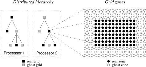
The code uses blockstructured adaptive mesh refinement (as described in section 6.1) to achieve high resolution. To parallelize the computation, a concept of ghost grids is used. The root grid is split into a number of grid patches, at least as many as the number of processors. Then, as grids are added, each grid is placed by default on the same processor as its parent. Once the rebuild of the hierarchy has been completed on a given level, the load balancing ratio between processors is computed and grids are transfered between processors in an attempt to even the load. However, the structure of the grid patch hierarchy is stored redundantly on every processor to ease communication. To allow for this, each real grid, which resides on only one processor, is represented by a ghost grid (which is a grid patch without data) on every other processor. This structure is shown graphically in figure 7.1.

Figure 7.1: Real and ghost grids in a hierarchy; real and ghost zones in a grid (Norman et al., 2007).

Enzo is publicly available from http://lca.ucsd.edu/software/enzo/. However to integrate and test our SGS model several modifications to the public version were necessary.

7.2 Modifications to Enzo

7.2.1 Turbulent energy as a color field

To implement the Schmidt model into Enzo, it was necessary to introduce a new field for the turbulent energy, which is advected by the PPM solver. To achieve this, we used the capability of Enzo to incorporate an arbitrary number of color fields³⁶³⁶See appendix I. into the simulation. Thus the turbulent energy field is implemented as another color field. Nevertheless it was necessary to change the default behavior of color fields in Enzo. By default, Enzo treats a color like a density. But since we want turbulent energy to be treated in analogy to the internal energy, which is implemented as specific quantity, we changed the treatment of color fields in our version of Enzo as to behave like a specific quantity.

7.2.2 Coupling of turbulent energy and time step restriction

The source/sink terms in the turbulent energy equation and the terms arising in the internal energy equation and the momentum equation due to our subgrid model are coupled to the fields in first order, which means for some arbitrary field $f$ at timestep $t_{n}$ , the source terms $s_{1},s_{2},\ldots$ are added in the following way

\displaystyle f_{n+1}=f_{n}+s_{1,n}\Delta t+s_{2,n}\Delta t+\ldots

(7.1)

where $\Delta t=t_{n+1}-t_{n}$ is the chosen timestep. But due to the low accuracy of the scheme, it might happen, that for a big timestep the value of one of the energy fields in a cell drops below zero, which is unphysical and numerically unstable. To account for that, we had to restrict the timestep in the code. We do this by applying the following estimator

\displaystyle\Delta t_{turb}=C_{turb}\min{\left(\sqrt{\frac{l_{\Delta}}{\left% \lvert\boldsymbol{a}_{turb}\right\rvert}}\right)},

(7.2)

where the minimum is taken over all cells of all grids on one level of refinement, the turbulent acceleration is $\boldsymbol{a}_{turb}=\frac{1}{\langle\rho\rangle}{\frac{\partial}{\partial r_% {j}}\hat{\tau}(v_{i},v_{j})}$ and $C_{turb}=0.05$ . If the so-estimated minimal allowed timestep due to our turbulent model $\Delta t_{turb}$ is smaller than the timestep computed by the other estimators in the code (e.g. estimator based on the CFL-criterion, for gravity and so on) it will be chosen as the timestep for the next iteration. This procedure ensures that even for big turbulent acceleration (which also means big source/sink terms) due to our turbulent model, our computation is numerically stable. Of course, there is one drawback to this procedure: if the turbulent acceleration becomes really huge, the timestep of the simulation will be extremely small, effectively stopping the simulation. This can only be circumvented by either using a higher accuracy scheme for coupling the sink/source terms to the equations or by using a different subgrid model, which does not produce numerically instable huge values of $\left\lvert\boldsymbol{a}_{turb}\right\rvert$ . The Sarkar corrections are a step in this direction, but further steps may be necessary in the future.

7.2.3 Transfer of turbulent energy at grid refinement/derefinement

By default, when a new finer grid gets created in Enzo, the values on the finer grid are generated by interpolating them from the coarser grid using a conservative interpolation scheme. At each timestep of the coarse grid, the values from the fine grid are averaged and replace the values computed on the coarse grid in the region where fine and coarse grid overlap. As already mentioned in section 6.3 these procedures must be modified in our approach to combine LES and AMR.

So at refinement we do the following:

1.

Interpolate the values from the coarse to the fine grid using standard interpolation scheme from Enzo.
2.

On the finer grid, correct the values of specific kinetic energy $e_{k}=\frac{1}{2}v^{2}$ , velocity components $v_{i}$ and specific turbulent energy $e_{t}=\frac{1}{2}q^{2}$ as follows

$\displaystyle e^{\prime}_{k}$ $\displaystyle=e_{k}+e_{t}{\left(1-r^{-2/3}\right)},$ (7.3)

$\displaystyle v^{\prime}_{i}$ $\displaystyle=v_{i}\sqrt{1+\frac{e_{t}}{e_{k}}{\left(1-r^{-2/3}\right)}},$ (7.4)

$\displaystyle e^{\prime}_{t}$ $\displaystyle=e_{t}-e_{t}{\left(1-r^{-2/3}\right)},$ (7.5)

where primed quantities are the final values on the fine grid.

At derefinement we reverse this procedure:

1.

Average the values from the fine grid and replace the corresponding values on the coarse grid
2.

On the coarse grid, correct the averaged values of kinetic energy, velocity components and turbulent energy

$\displaystyle e^{\prime}_{t}$ $\displaystyle=e_{t}+e_{t}{\left(r^{2/3}-1\right)},$ (7.6)

$\displaystyle v^{\prime}_{i}$ $\displaystyle=v_{i}\sqrt{1-\frac{e_{t}}{e_{k}}{\left(r^{2/3}-1\right)}},$ (7.7)

$\displaystyle e^{\prime}_{k}$ $\displaystyle=e_{k}-e_{t}{\left(r^{2/3}-1\right)}.$ (7.8)

Here primed quantities denote the final values on the coarse grid.

It should be noted that derefinement with this procedure is only possible if there is enough kinetic energy on the fine grid, because on the coarse grid, we must have $e^{\prime}_{k}\geq 0$ . This is only the case for

\displaystyle\frac{e_{t}}{e_{k}}\leq{\left(r^{2/3}-1\right)}.

(7.9)

For example for a refinement ratio $r=2$ this yields $e_{k}\geq 0.58e_{t}$ . So if this criterion is not satisfied, we do not correct the values of the energies and velocities at derefinement.³⁷³⁷One might ask, why not do the correction step before the interpolation/averaging step, since that might produce less noise. The reason for our choice was, that otherwise we would had to introduce an additional temporary field into the code, which would lower the performance.

7.2.4 Random forcing

To simulate driven turbulent flow, a random forcing mechanism was implemented into our version of Enzo. The forcing field is generated by a stochastic differential equation called Ornstein-Uhlenbeck process (Schmidt, 2004). This process generates a temporally and spatially varying force field which acts on the fluid. The components of the force are generated in Fourier space, because there it is easier to split the force field into a solenoidal and a dilatational (compressive) part.³⁸³⁸Also called Helmholtz decomposition, see Schmidt (2004). Hence the force field is characterized by a weight $\zeta$ , which is zero, if the force field is purely compressive (which means it will not directly generate any vorticity), and one, if the force field is purely solenoidal (which means it will not directly generate any divergence in the velocity field). The strength of the force field is characterized by a forcing Mach number $M_{f}$ , which is loosely connected to the mean Mach number reached in the simulation after one integral time

\displaystyle t_{int}=\frac{l_{0}}{M_{f}\langle c_{s}\rangle},

(7.10)

where $l_{0}$ is the mean driving length scale size and $\langle c_{s}\rangle$ is the mean sound speed. The force field is adjusted to drive the fluid only on length scales around the characteristic forcing length $l_{0}=\frac{l_{box}}{\alpha_{f}}$ with $\alpha_{f}=2$ to allow for an undisturbed generation of the energy dissipation cascade down to smaller scales.

7.2.5 Statistics tool

To be able to extract and analyze statistical quantities from the simulation, sophisticated routines have been implemented, which allow us to compute mass weighted and normal mean values, standard deviations and root mean square values at every cycle for each quantity and for each level of an AMR simulation. We make heavy use of these routines in the following sections.

7.3 Energy conservation

Global conservation of energy in a fluid code with a SGS model like the Schmidt model is not achieved easily. This is because of the nonlocal features of this model. As shown in chapter 4, the equation of turbulent energy (4.29) is generated by subtracting the equation of resolved kinetic energy (4.30) from the filtered equation of turbulent energy 4.6. In other words, the sum of turbulent energy equation and resolved energy equation must yield the filtered kinetic energy equation. In particular, the sum of turbulent production term $\hat{\tau}(v_{j},v_{i})\frac{\partial}{\partial r_{j}}\hat{v_{i}}$ and resolved kinetic energy reduction term $\hat{v}_{i}\frac{\partial}{\partial r_{j}}\hat{\tau}(v_{i},v_{j})$ must add up to the corresponding flux term in the filtered equation of kinetic energy

\displaystyle\frac{\partial}{\partial r_{j}}\hat{v}_{i}\hat{\tau}(v_{i},v_{j})% =\hat{v}_{i}\frac{\partial}{\partial r_{j}}\hat{\tau}(v_{i},v_{j})+\hat{\tau}(% v_{j},v_{i})\frac{\partial}{\partial r_{j}}\hat{v_{i}}.

(7.11)

This is important, since we know that the integral of the flux term over the whole volume must be zero

\displaystyle\int\frac{\partial}{\partial r_{j}}\hat{v}_{i}\hat{\tau}(v_{i},v_% {j})dV=\oint\hat{v}_{i}\hat{\tau}(v_{i},v_{j})dA=0.

(7.12)

But this is not guaranteed numerically, if we compute the turbulent production term and the kinetic energy reduction term independent of each other, since small numerical errors might lead to a violation of equation (7.11) locally, which leads to a big violation of equation (7.12) globally.

We therefore compute the resolved kinetic energy reduction term indirectly as

\displaystyle\hat{v}_{i}\frac{\partial}{\partial r_{j}}\hat{\tau}(v_{i},v_{j})% =\frac{\partial}{\partial r_{j}}\hat{v}_{i}\hat{\tau}(v_{i},v_{j})-\hat{\tau}(% v_{j},v_{i})\frac{\partial}{\partial r_{j}}\hat{v_{i}},

(7.13)

since this will guarantee, that equation (7.12) is fullfilled globally. We found that the global energy is thus much better conserved.

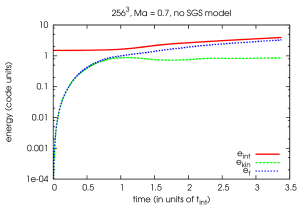
In the following we present our results on energy conservation. The analyzed simulation of driven turbulence has a static grid of size 1.0 (in code units) with a resolution of $256^{3}$ grid points and periodic boundary conditions. At time $t=0$ the baryonic fluid is at rest. The fluid is driven by random forcing as described in section 7.2.4 with $\zeta=1.0$ and $M_{f}=0.68$ . The simulation is adiabatic (the adiabatic index $\gamma=\frac{5}{3}$ ) and uses none of the features necessary for a cosmological simulation (comoving coordinates, selfgravity, dark matter …) except dual energy formalism. The mean sound speed of the simulation is $c_{s}=\sqrt{\gamma}$ , since the mean pressure and density are set to one in code units.

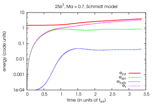
The plots a and b show the typical time development of the mass weighted mean energies in our simulation including the energy injected into the system by random forcing. It is evident from the curve of the turbulent energy, that after one integral time scale, our simulation reaches a equilibrium between production and dissipation of turbulent energy.

Figure 7.3: Relative error of total energy in the simulation.

In figure 7.3 we plotted the time development of the relative error $\frac{\Delta e(t)}{e(0)}$ of the mean total energy, which is the sum of the mass weighted means of internal energy, kinetic energy, turbulent energy minus the injected energy due to the forcing

\displaystyle\hat{e}_{tot}=\hat{e}_{int}+\hat{e}_{kin}+\hat{e}_{t}-\hat{e}_{f},

(7.14)

where $\hat{e}=\frac{\langle\rho e\rangle}{\langle\rho\rangle}$ . It demonstrates, that with our Schmidt model, the relative error in energy is comparable to the error without SGS model and is around 1%. Also the energy conserving properties of the Sarkar model are equally good.

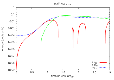
Figure 7.4: Differences in energies between simulation with and without SGS model, compared to the time development of the turbulent energy.

It is also instructive to plot the difference between internal energy of the simulation without the SGS model and the internal energy with the Schmidt model and the difference between the kinetic energies of both simulations. These differences are shown in figure 7.4. One can conclude from this figure, that, at the beginning of the turbulent driving, the turbulent energy produced in our simulation with SGS is found in the kinetic energy of the simulation without SGS. From $t=1.2\ t_{int}$ on most of the turbulent energy can be found in the internal energy of the simulation without SGS. Turbulent energy can therefore be interpreted as a kind of buffer, which prevents the kinetic energy in our simulation to be converted instantly into thermal energy.

7.4 Scaling of turbulent energy

In our $\epsilon$ -based approach to combine AMR and LES we assumed that the turbulent energy scales according to equation $\eqref{eq:qscale}$ like $q^{2}\sim l^{2/3}$ . We conducted several simulations of driven turbulence to check the validity of this assumption.

The simulations were done on a static grid in a computational domain of size 1.0 with periodic boundary conditions. At time $t=0$ the baryonic fluid is at rest. The fluid is driven by random forcing as described in section 7.2.4 with $\zeta=0$ (purely solenoidal forcing). The simulations were done for nearly isothermal gas ( $\gamma=1.01$ ) with mean pressure and density set to $1.0$ in code units. We used forcing Mach numbers of $M_{f}=0.2$ and $M_{f}=0.68$ and varied the resolution from $32^{3}$ to $256^{3}$ grid points. For $M_{f}=0.68$ the simulations were transonic reaching reaching a Mach number around one (see figure 7.5).

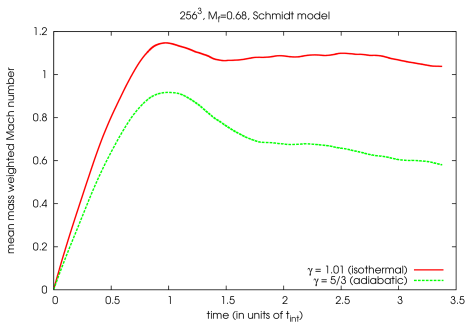
Figure 7.5: Mean Mach number for adiabatic and isothermal simulation using an equal forcing Mach number $M_{f}=0.68$ .

The characteristic time development of the turbulent energy dependent on the resolution of the simulation can be seen in figures a - d.

We compute mean turbulent energies by averaging the turbulent energy from $t=3.0\ t_{int}$ to the end of the simulation and plot them against the resolution of the simulation. The results together with a power-law fit are shown in figures a and b. From this we see that for a low Mach number forcing our assumption $q^{2}\sim l^{2/3}$ ( $l$ is indirect proportional to the resolution) is fulfilled indeed. Nevertheless for high Mach number flows the scaling of turbulent energy becomes steeper and is $q^{2}\sim l^{0.77}$ for the Schmidt model and $q^{2}\sim l^{0.71}$ for the Sarkar model. In other words for higher Mach number flows, our correction of turbulent energy at grid refinement/derefinement based on relation $\eqref{eq:qscale}$ should probably be seen only as a good guess of the initial values of turbulent energy on the finer/coarser grid. Also we conclude that for higher Mach number flows one should use the Sarkar corrections to the Schmidt model, since this leads to a scaling of turbulent energy more similar to the incompressible low Mach number case.

7.5 Comparison of static grid to AMR turbulence simulations

Figure 7.8: Thick lines: mean mass weighted turbulent energy for each level of the AMR simulation using our procedure of transferring turbulent energy at grid refinement/derefinement. Thin lines: the corresponding development of turbulent energy of the static grid simulations.

Figure 7.9: Thick lines: mean mass weighted turbulent energy for each level of the AMR simulation without transferring turbulent energy at grid refinement/derefinement. Thin lines: the corresponding development of turbulent energy of the static grid simulations.

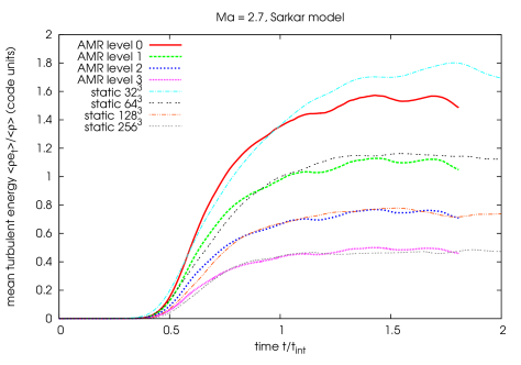
To be consistent the results of an AMR simulation in the limit of complete refinement of the whole computational domain should resemble the results of a corresponding static grid simulation. To test this, we compared an AMR simulation with a $32^{3}$ root grid resolution and three additional levels with a refinement factor of 2 between each level, covering the whole domain, with the corresponding static grid simulations of driven turbulence with resolutions of $32^{3},64^{3},128^{3}$ and $256^{3}$ .

Again the simulations were done in a computational domain of size 1.0 with periodic boundary conditions. At time $t=0$ the baryonic fluid is at rest. The fluid is driven by random forcing as described in section 7.2.4 with $\zeta=0$ (purely solenoidal forcing). The simulations were done for nearly isothermal gas ( $\gamma=1.01$ ) with mean pressure and density set to $1.0$ in code units. We used a forcing Mach number of $M_{f}=2.7$ and therefore used the SGS model with Sarkar corrections.

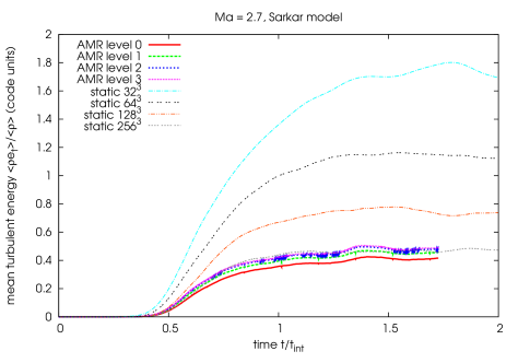
The results of this consistency check can be seen in figure 7.8. We observe that the time development of the mean turbulent energy in this simulation of supersonic driven turbulence simulation is very similar on the different levels of the AMR simulation compared with the static grid simulations, except for some deviations at the root level. But comparing these results to a simulation without correcting turbulent energy at grid refinement/derefinement (figure 7.9), it is evident that our $\epsilon$ -based approach of turbulent energy transfer is much more consistent with the static simulations of driven turbulence.

$\displaystyle e^{\prime}_{k}$	$\displaystyle=e_{k}+e_{t}{\left(1-r^{-2/3}\right)},$	(7.3)
$\displaystyle v^{\prime}_{i}$	$\displaystyle=v_{i}\sqrt{1+\frac{e_{t}}{e_{k}}{\left(1-r^{-2/3}\right)}},$	(7.4)
$\displaystyle e^{\prime}_{t}$	$\displaystyle=e_{t}-e_{t}{\left(1-r^{-2/3}\right)},$	(7.5)

$\displaystyle e^{\prime}_{t}$	$\displaystyle=e_{t}+e_{t}{\left(r^{2/3}-1\right)},$	(7.6)
$\displaystyle v^{\prime}_{i}$	$\displaystyle=v_{i}\sqrt{1-\frac{e_{t}}{e_{k}}{\left(r^{2/3}-1\right)}},$	(7.7)
$\displaystyle e^{\prime}_{k}$	$\displaystyle=e_{k}-e_{t}{\left(r^{2/3}-1\right)}.$	(7.8)