Time Series Prediction Part I

Dr. Andreas Maier

2022-07-21

Time Series

Clustering
- Dynamic Time Warping
Segmentation
- Speech recognition
Classification
Anomaly/Outlier Detection
Imputation
Forecasting
- Trajectory prediction
- Stock Market prediction

Univariate
Multivariate
Zerovariate
- Delphi Method

“Prediction is the essence of intelligence, and that’s what we’re trying to do.”

– Yann LeCun (2015)

“Prediction is very difficult, especially if it’s about the future!”

– Niels Bohr

“What we can’t predict, we call randomness.”

– Albert Einstein

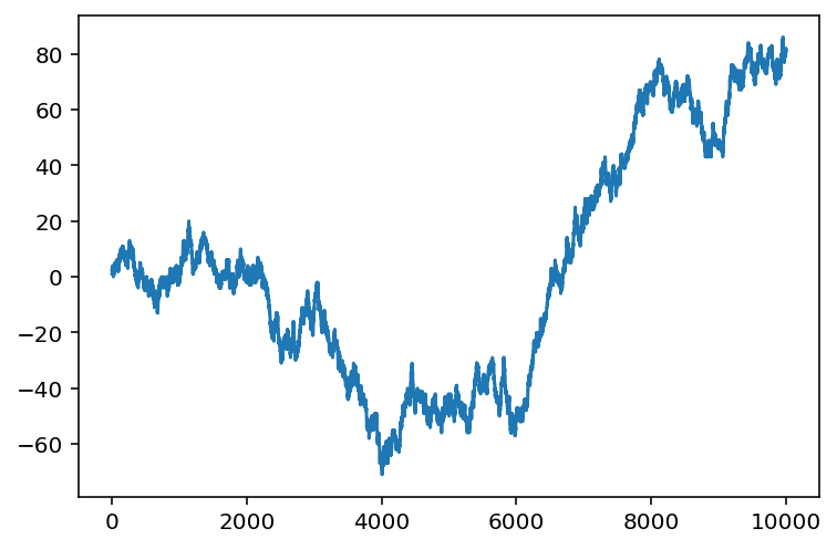
Understanding Randomness 1

Random walk: cumulative sum of random numbers

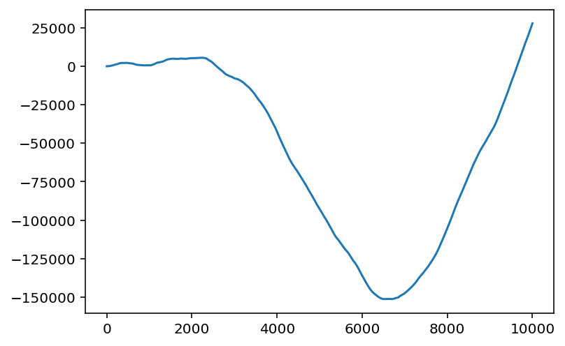
Understanding Randomness 2

Walk of random walk: cumulative sum of a random walk

Wat??

https://stats.stackexchange.com/questions/580718/properties-of-cumulative-sum-of-a-random-walk

Pearson correlation coefficient \(r\)

Measures linear correlation between two sets of data
Equal to the slope of a linear regression model (for standardized data \(\sigma_x=\sigma_y=1\))¹

\[ \hat{y} = \phi_0 + \phi_1 x = \phi_0 + \frac{cov(x,y)}{\sigma_x^2} x = \phi_0 + r \frac{\sigma_x}{\sigma_y} x \]

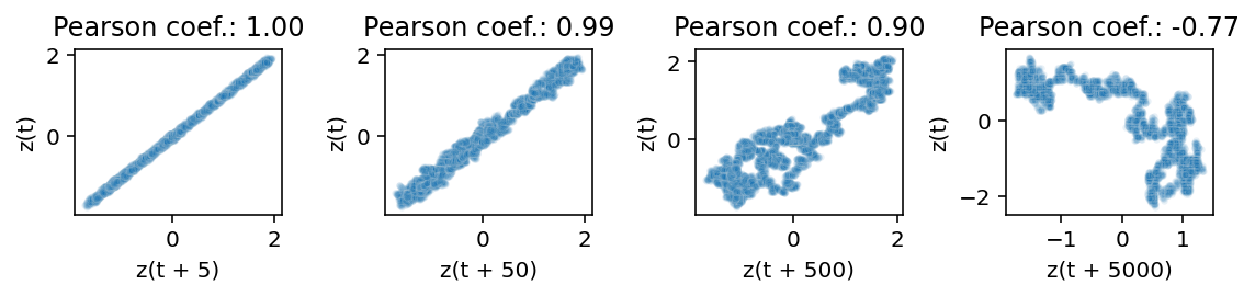
Autocorrelation 1

Pearson coefficients between time series and time shifted version of itself

Autocorrelation 2

ACF (auto correlation function) of non-stationary data decreases slowly²
random walk is non-stationary

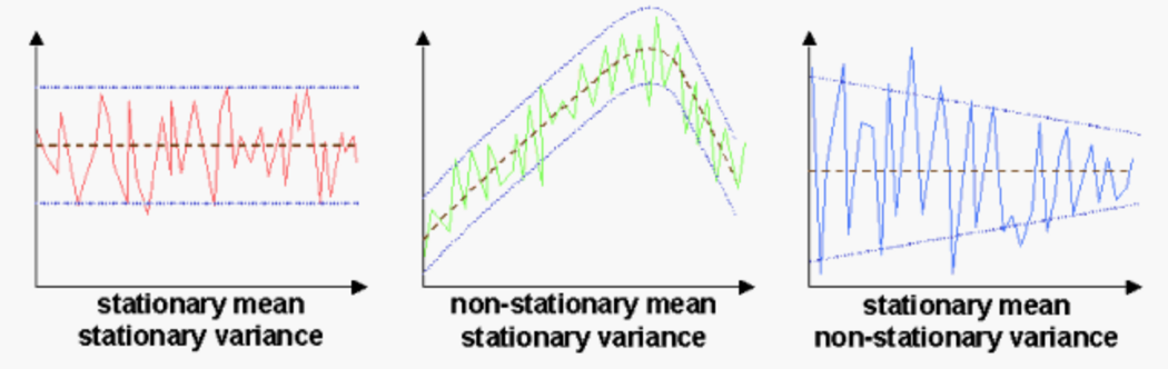
Stationarity

Statistical properties don’t change over time

A stationary time series has no seasonality or trend.
Many tools, statistical tests and models (ARIMA!) rely on stationarity.

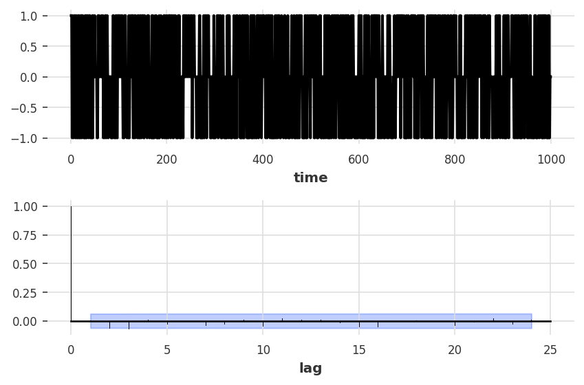
Differencing

Differencing of degree \(d\) can help to stabilise the mean eliminating/reducing trend and seasonality.
Transformations such as logarithms can help to stabilise the variance
ACF is zero for first derivative of random walk

Partial autocorrelation 1

Direct linear correlation \(r_k\) between \(y\) and \(x_k\) \[ \hat{y} = \phi_0 + 0 \cdot x_1 + ... + r_k x_k \]
Partial correlation \(p_k\) between \(y\) and \(x_k\) \[ \hat{y} = \phi_0 + \phi_1 x_1 + ... + p_k x_k \] Dependency on \(x_1, x_2, ...\) is absorbed into \(\phi_1, \phi_2, ...\)

Partial correlation is linear correlation between \(y\) and \(x_k\) with indirect correlation to \(x_1, x_2, ...\) removed.⁴

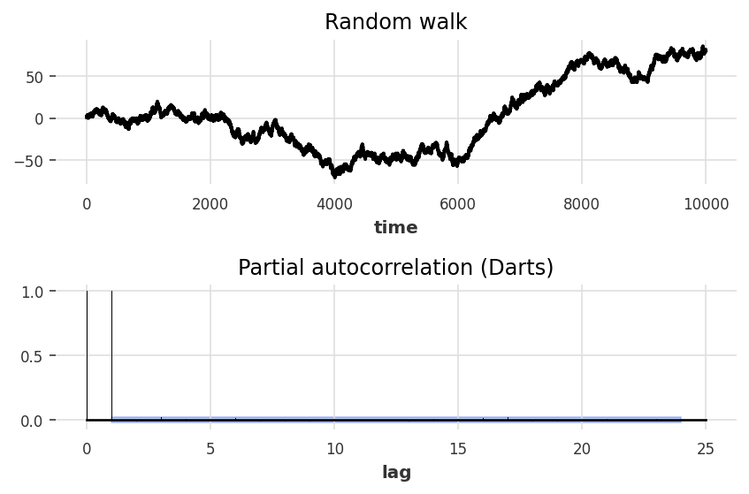
Partial autocorrelation 2

PACF (Partial autocorellation function) is zero for random walk except for lag 1

Autoregression model

forecast \(y_t\) using a linear combination of past values \[ \hat{y}_t = \phi_0 + \phi_1 y_{t-1} + \phi_2 y_{t-2} + ... + \phi_p y_{t-p} \]
Autoregression means linear regression with lagged version of itself (similar to autocorrelation)
AR(p) means \(\phi_0, ..., \phi_p \neq 0\)
Autoregressive process can be used to generate data from random white noise \(\epsilon_t\) and fixed parameters \(\phi_k\) \[ y_t = \epsilon_t + \phi_0 + \phi_1 y_{t-1} + \phi_2 y_{t-2} + ... + \phi_p y_{t-p} \]
For \(\phi_0 = 0\) and \(\phi_1=1\) an AR(1) process is a random walk

Moving average model

The name “moving average” is technically incorrect ⁵
Better would be lagged error regression
forecast \(y_t\) using a linear combination of past forecast errors \[ \hat{y}_t = \theta_0 + \theta_1 \epsilon_{t-1} + \theta_2 \epsilon_{t-2} + ... + \theta_q \epsilon_{t-q} \]
MA(q) cannot be fitted like an ordinary least square (OLS), because the forecast errors are not known
Example algorithm: Set initial values for \(\theta_k\) and \(\epsilon_k\), then
- For i=1..N do
  1. Compute error terms for all \(t\): \(\epsilon_t\) = \(y_t - \hat{y}_t\)
  2. Run a regression of \(y_t\) against \(\hat{y}_t\) and update \(\theta_k\)
  3. Repeat
Like(?) Iteratively_reweighted_least_squares or similar iterative process to estimate \(\theta_k\)

ARIMA

Autoregressive integrated moving average model combines AR(p), differencing/integrating I(d) and MA(q) \[ \hat{y}_t = c + \phi_1 y^{(d)}_{t-1} + ... + \phi_p y^{(d)}_{t-p} + \theta_1 \epsilon_{t-1} ... + \theta_q \epsilon_{t-q} \]

Model	equivalent to
ARIMA(0,1,0)	Random Walk (with drift)
ARIMA(0,1,1)	simple exponential smoothing ETS(A,N,N)
ARIMA(1,0,0)	discrete Ornstein-Uhlenbeck process ⁶

To find the best fitting ARIMA model one can use the Box-Jenkins-Method

Box-Jenkins Method

Make the time series stationary (e.g. standardization, differencing \(d\)-times, …)
Use ACF plot and PACF plot to identify the parameter \(p\) and \(q\)
Fitting the parameters of the ARIMA(p,d,q) model. This can be done with Hannan–Rissanen (1982) algorithm
1. AR(m) model (with \(m > max(p, q)\)) is fitted to the data
2. Compute error terms for all \(t\): \(\epsilon_t\) = \(y_t - \hat{y}_t\)
3. Regress \(y_t\) on \(y^{(d)}_{t-1},..,y^{(d)}_{t-p},\epsilon_{t-1},...,\epsilon_{t-q}\)
4. To improve accurancy optinally regress again with updated \(\phi,\theta\) from step 3
Other algorithms (maximizing likelihood) are often used in practice ⁷ ⁸
Statistical model checking (analysis of mean, variance, (partial) autocorrelation, Ljung–Box test of residuals)
Once the residuals look like white noise, do the forecast

Nowadays all these steps are automated by tools like AutoARIMA etc.

Why???

Why combine AR and MA ?
- Wold’s theorem ?
AR is analogeous to linear regression, but what is MA analogeous to outside of time series analysis?
Why is ARIMA better than AR alone?